Rice
Data
Input data description
- ricepan.gff (35M, 50995 genes):Annotation file for the rice pan-genome.
- ricepan.chrl (0.4K):File recording chromosome lengths of the rice pan-genome.
- rice.pheno (13K, 453 samples, 3 phenotypes):Phenotype information file for rice samples.
- rice_bam/ (5.44TB, 453 samples):Directory storing alignment results.
Data download
mkdir data && cd data;
wget "https://cgm.sjtu.edu.cn/APAV/data/rice/ricepan.gff.gz" && gunzip ricepan.gff.gz
wget "https://cgm.sjtu.edu.cn/APAV/data/rice/ricepan.chrl"
wget "https://cgm.sjtu.edu.cn/APAV/data/rice/rice.pheno"
cd ..
## The BAM files are too large to download. These files are primarily used for calculating coverage in Step 2. You can directly download the coverage calculation results for subsequent analysis.
wget https://cgm.sjtu.edu.cn/APAV/case/rice/ricepan.cov && wget https://cgm.sjtu.edu.cn/APAV/case/rice/ricepan_ele.cov
Code and Result
1. Coordinate Extraction
Extract genomic coordinates for genes and genetic elements from GFF annotation files:apav gff2bed --gff data/ricepan.gff --chrl data/ricepan.chrlOutput: ricepan.bed
2. Coverage Calculation
Calculate coverage for gene and element regions across all samples based on alignment results, using the transcript with the longest CDS region as the representative transcript for the gene:apav staCov --bed ricepan.bed --bamdir data/rice_bam --asgene --rep cdslen ## This step will consume a lot of time and you can download the results directly: wget https://cgm.sjtu.edu.cn/APAV/case/rice/ricepan.cov && wget https://cgm.sjtu.edu.cn/APAV/case/rice/ricepan_ele.covOutput: ricepan.cov, ricepan_ele.cov
3. PAV Determination
Determine gene PAV at 50% threshold (genes with coverage ≥50% are classified as "presence", otherwise "absence"):apav callPAV --cov ricepan.cov --pheno data/rice.pheno --thre 0.5Output:ricepan_all.pav(raw PAV matrix), ricepan_dispensable.pav(non-core gene subset)
Determine element PAV at 50% threshold:
apav callPAV --cov ricepan_ele.cov --pheno data/rice.pheno --thre 0.5Output: ricepan_ele_all.pav, ricepan_ele_dispensable.pav
Remove genes absent across all samples:
awk '{if ($1 ~ /^#/) {print; next}; for (i=6; i<=NF; i++) if ($i != 0) {print; next};}' ricepan_all.pav > ricepan.pav
awk '{if ($1 ~ /^#/) {print; next}; for (i=6; i<=NF; i++) if ($i != 0) {print; next};}' ricepan_dispensable.pav > ricepan_dis.pav
Output: ricepan.pav, ricepan_dis.pav
4. Pangenome Size Estimation
Extract grouping information from the phenotype file:cat data/rice.pheno | cut -f 1,2 > rice.groupOutput: rice.group
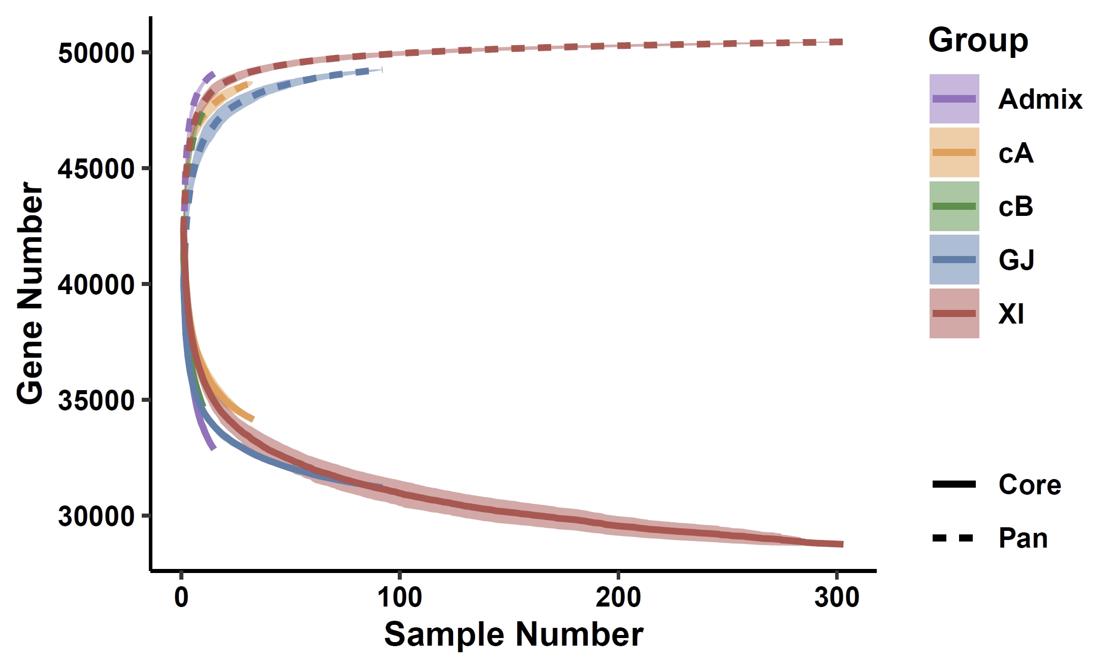
Estimate pan-genome size by group:
apav pavSize --pav ricepan.pav --group rice.group --out rice_grouped.sizeOutput: rice_grouped.size
Plot the size curve:
apav pavPlotSize --size rice_grouped.size --path_color '#9a71c1,#ea9e4a,#4d9242,#5880ae,#b7514d' --ribbon_fill '#9a71c1,#ea9e4a,#4d9242,#5880ae,#b7514d' --y_title "Gene Number" --fig_height 3 --fig_width 5Output: rice_grouped_size_curve.pdf
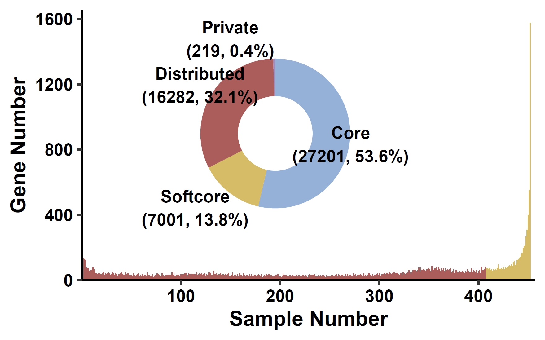
5. PAV analysis
Classify genes into core, soft-core, distributed, and private categories:apav pavPlotHist --pav ricepan.pav --y_title "Gene Number" --ring_r 0.45 --ring_label_size 3 --fig_height 2.5 --fig_width 4Output: ricepan_pav_hist.pdf
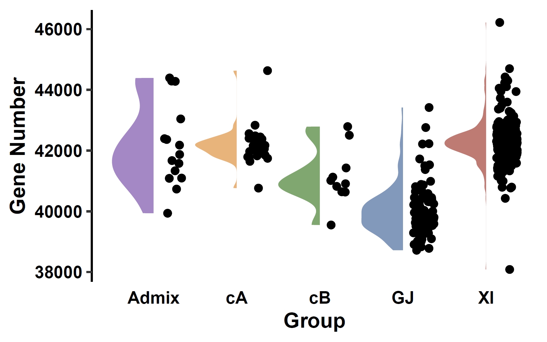
Compare gene counts across phenotype groups:
apav pavPlotStat --pav ricepan.pav --pheno data/rice.pheno --add_pheno_info Group --y_title "Gene Number" --pheno_info_colors '#aa88cb,#f2b372,#76aa6a,#7e9bc0,#cb7871' --fig_width 4 --fig_height 2.5Output: ricepan_pav_sta.pdf
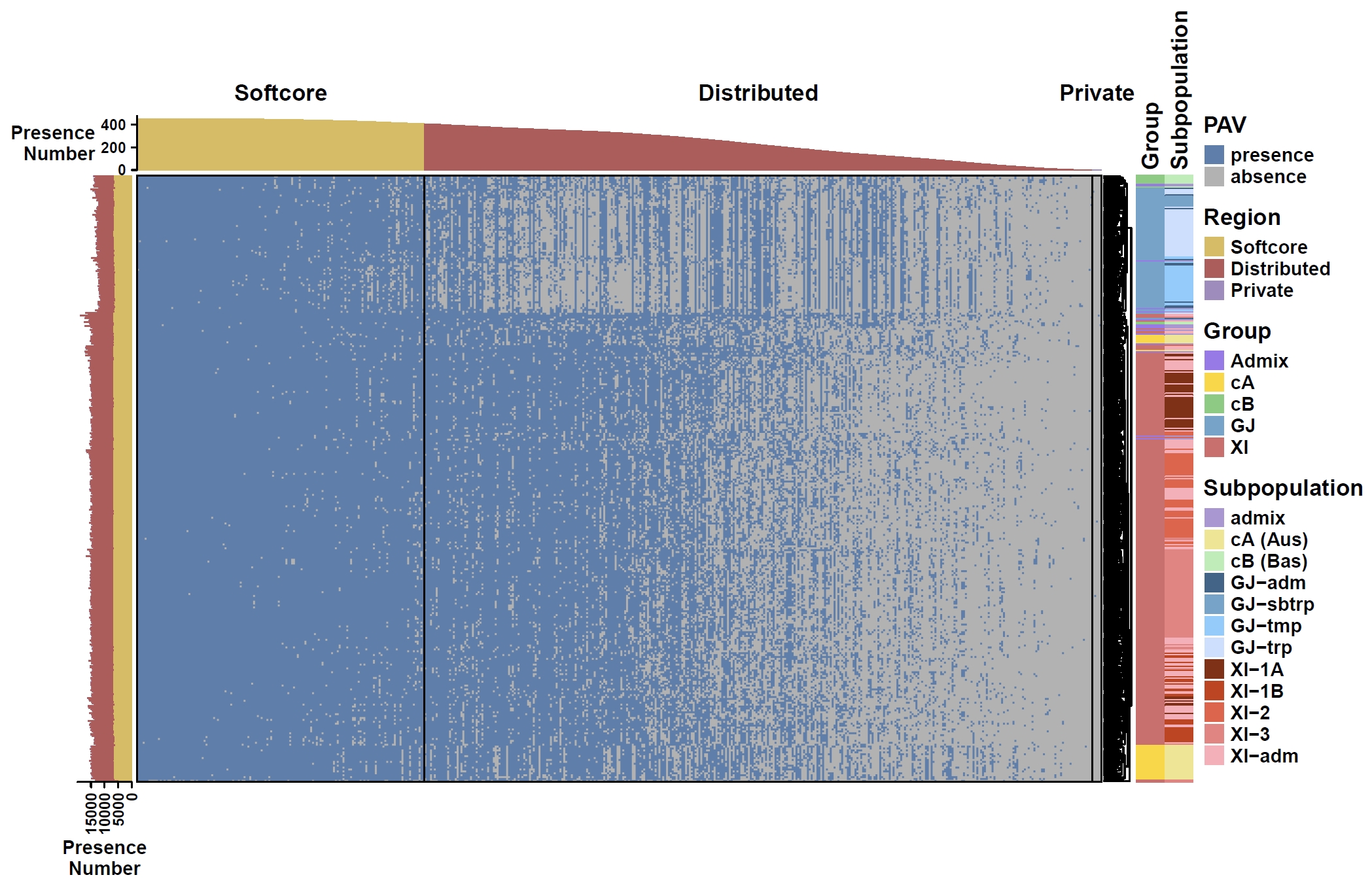
Plot heatmap for non-core genes:
cat data/rice.pheno | cut -f 1,2,3 > rice.anno
apav pavPlotHeat --pav ricepan_dis.pav --pheno rice.anno --cluster_rows --row_dend_side right --pheno_info_color_list Group=#9F79EE,#FFD700,#7CCD7C,#6CA6CD,#D66B6B --pheno_info_color_list Subpopulation=#AD98D6,#F0E68C,#B4EEB4,#36648B,#6CA6CD,#87CEFF,#CAE1FF,#8B2500,#CD3700,#EE5C42,#F08080,#FFAEB9 --fig_width 10 --fig_height 6.5
Output: ricepan_dis_pav_heatmap.pdf
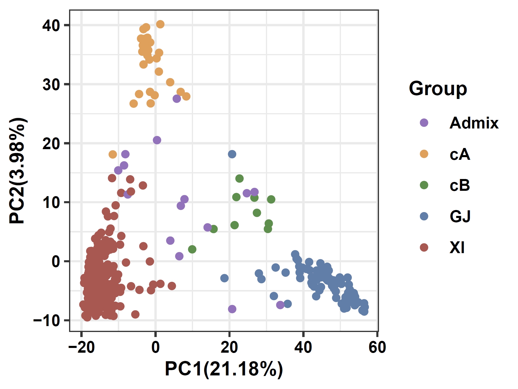
PCA based on non-core gene PAV:
apav pavPCA --pav ricepan_dis.pav --pheno data/rice.pheno --add_pheno_info Group --pheno_info_colors '#9a71c1,#ea9e4a,#4d9242,#5880ae,#b7514d' --fig_height 3 --fig_width 4Output: ricepan_dis_pav_pca.pdf
6. Phenotype Association Analysis
Calculate associations between non-core genes and phenotypes:apav pavStaPheno --pav ricepan_dis.pav --pheno data/rice.phenoOutput: ricepan_dis.phenores
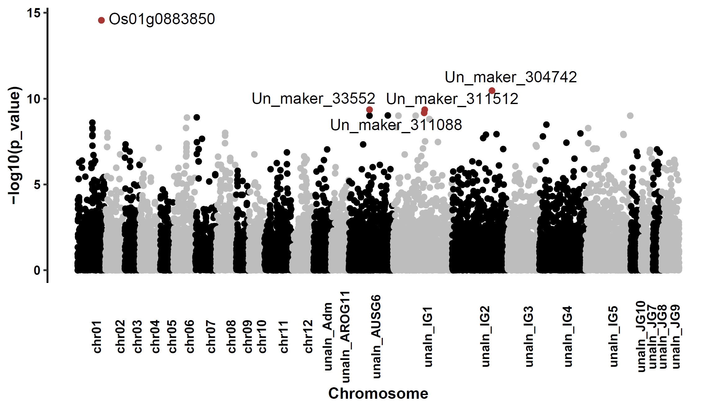
Manhattan plot for continuous phenotypes (e.g., plant height):
apav pavPlotPhenoMan --pav ricepan_dis.pav --pheno data/rice.pheno --pheno_res ricepan_dis.phenores --pheno_name Height --x_text_angle 90 --fig_height 4 --fig_width 7Output: ricepan_dis_pheno_Height_manhattan.pdf
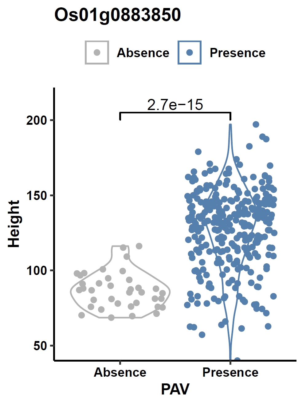
Visualize the association between gene PAV and a continuous phenotype (e.g., the Os01g0883850 gene and plant height) in a violin plot:
apav pavPlotPhenoVio --pav ricepan.pav --pheno data/rice.pheno --pheno_name Height --region_name Os01g0883850 --fig_height 4 --fig_width 3Output: ricepan_pheno_Height_Os01g0883850_violin.pdf
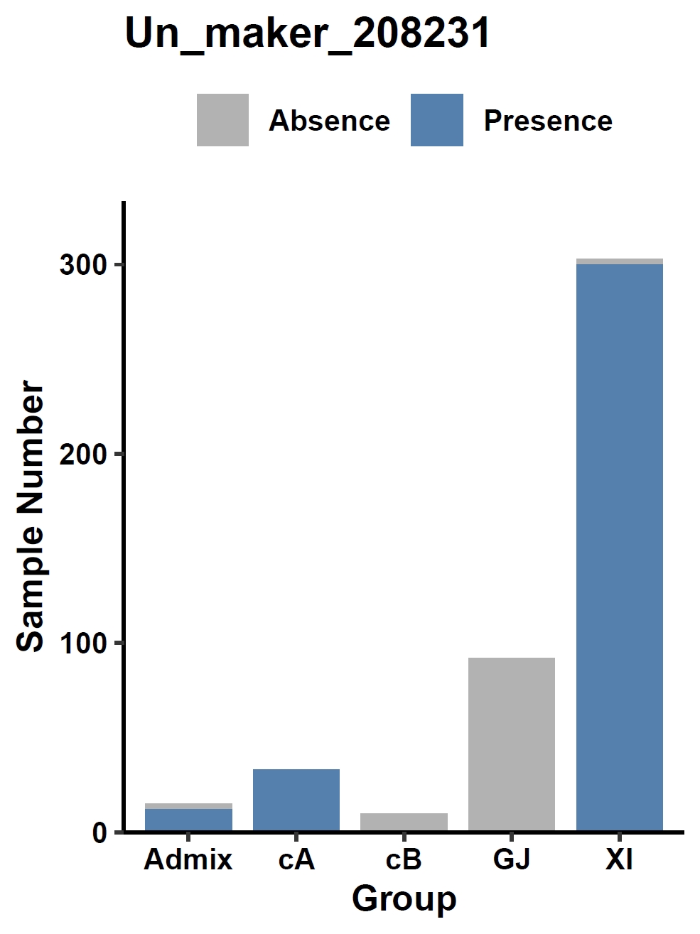
Visualize the association between a gene and a discrete phenotype (e.g., the Un_maker_208231 gene and accession group) in a bar plot:
apav pavPlotPhenoBar --pav ricepan.pav --pheno data/rice.pheno --pheno_name Group --region_name Un_maker_208231 --fig_height 4 --fig_width 3Output: ricepan_pheno_Group_Un_maker_208231_bar.pdf
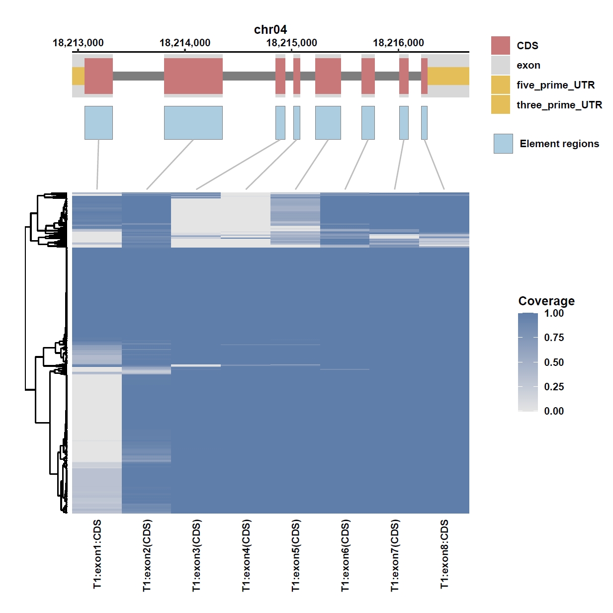
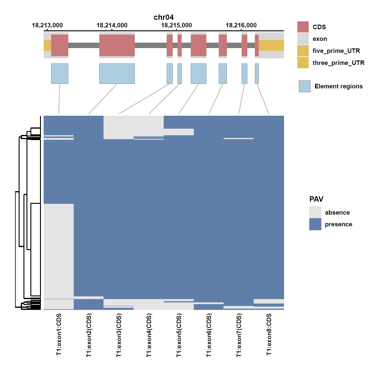
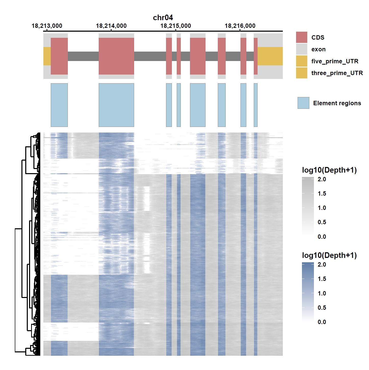
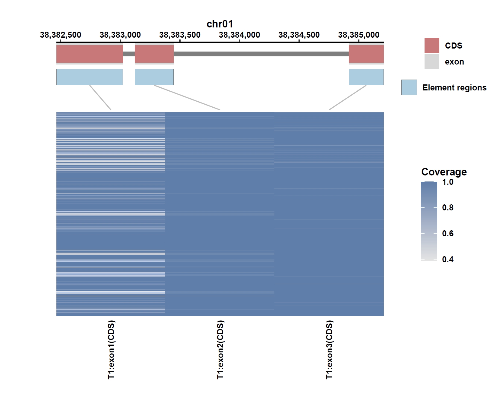
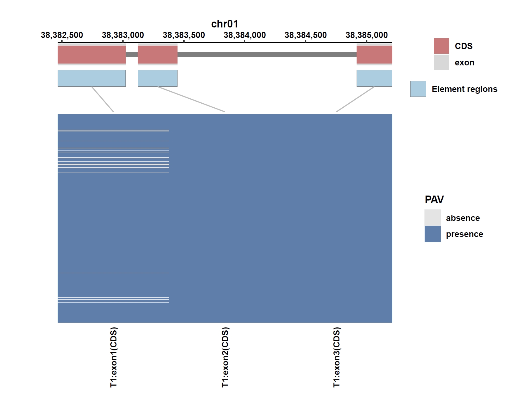
7. Element Visualization (Os04g0373400)
Prepare annotation and data files:mkdir ele_example_mate && cd ele_example_mate grep 'Os04g0373400' ../data/ricepan.gff > Os04g0373400.gff grep -E 'Annotation|Os04g0373400' ../ricepan_ele.cov > Os04g0373400.elecov grep -E 'Annotation|Os04g0373400' ../ricepan_ele_all.pav > Os04g0373400.elepavOutput: Os04g0373400.gff, Os04g0373400.elecov, Os04g0373400.elecov
Plot coverage, PAV and depth:
apav elePlotCov --elecov Os04g0373400.elecov --gff Os04g0373400.gff --cluster_samples --hide_sample_name --top_anno_height 0.3 --fig_width 7.5 --fig_height 7.5
apav elePlotPAV --elepav Os04g0373400.elepav --gff Os04g0373400.gff --cluster_samples --hide_sample_name --top_anno_height 0.3 --fig_width 7.5 --fig_height 7.5
apav elePlotDepth --ele Os04g0373400.elecov --bamdir ../data/rice_bam/ --gff Os04g0373400.gff --cluster_samples --hide_sample_name --log10 --top_anno_height 0.3 --fig_width 7.5 --fig_height 7.5
Output: Os04g0373400.elecov.pdf, Os04g0373400.elepav.pdf, Os04g0373400.elecov.depth.pdf
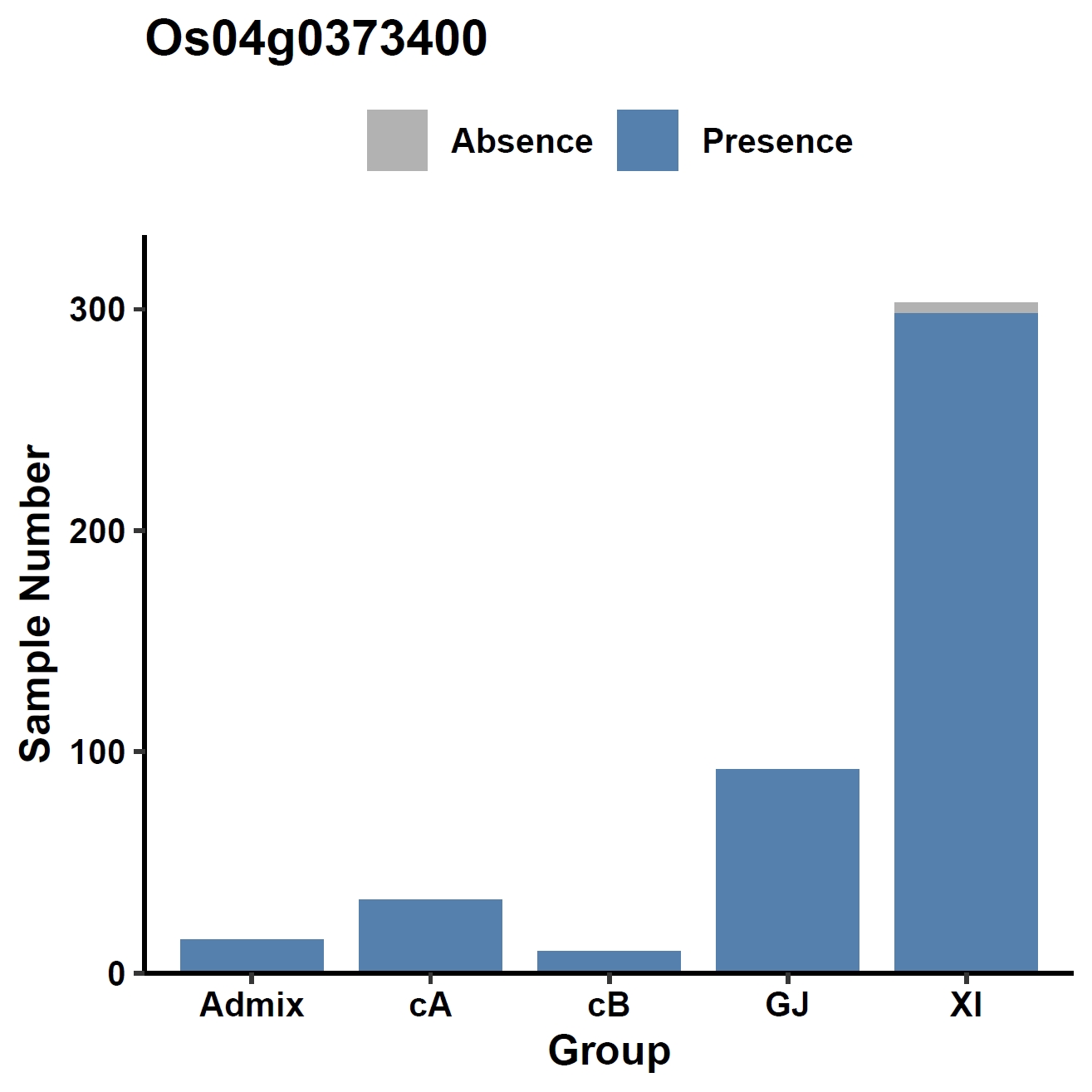
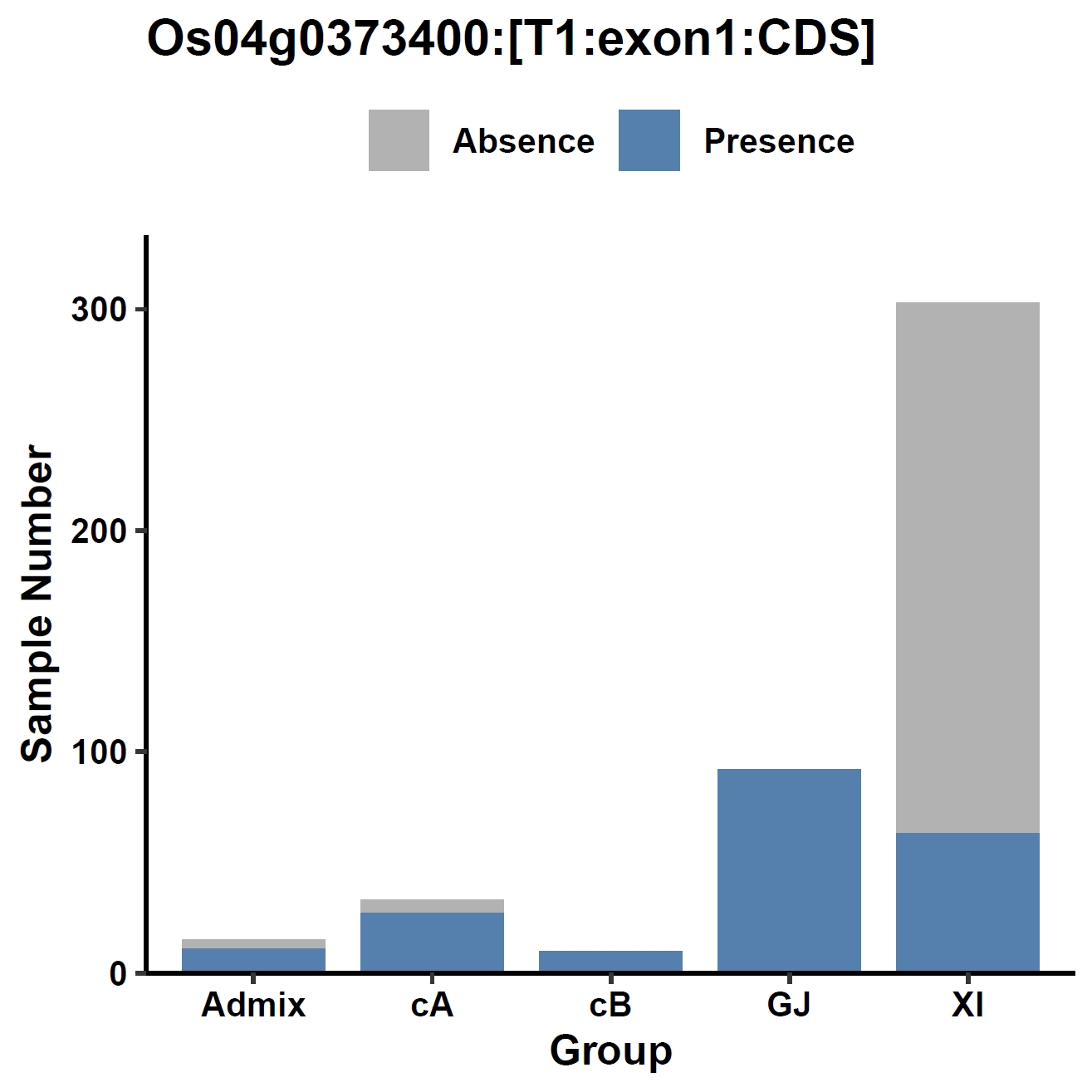
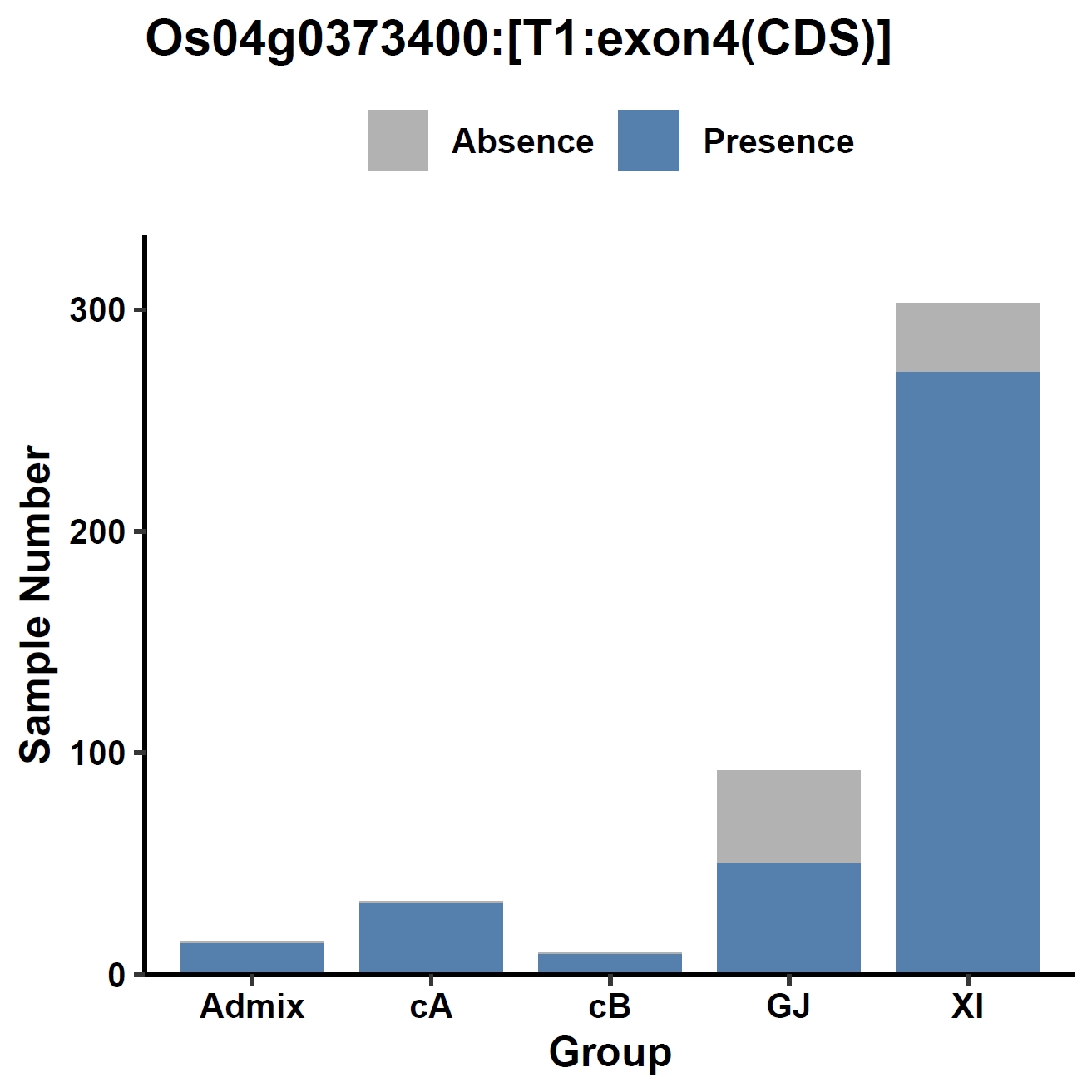
View phenotype association with group classification for gene and specific exons:
apav pavPlotPhenoBar --pav ../ricepan.pav --pheno ../data/rice.pheno --pheno_name Group --region_name Os04g0373400 --fig_width 4 --fig_height 4 --out Os04g0373400_group
apav pavPlotPhenoBar --pav Os04g0373400.elepav --pheno ../data/rice.pheno --pheno_name Group --region_name 'Os04g0373400:[T1:exon1:CDS]' --fig_width 4 --fig_height 4 --out Os04g0373400_group_exon1
apav pavPlotPhenoBar --pav Os04g0373400.elepav --pheno ../data/rice.pheno --pheno_name Group --region_name 'Os04g0373400:[T1:exon3(CDS)]' --fig_width 4 --fig_height 4 --out Os04g0373400_group_exon3
apav pavPlotPhenoBar --pav Os04g0373400.elepav --pheno ../data/rice.pheno --pheno_name Group --region_name 'Os04g0373400:[T1:exon4(CDS)]' --fig_width 4 --fig_height 4 --out Os04g0373400_group_exon4
cd ..
Output: Os04g0373400_group.pdf, Os04g0373400_group_exon1.pdf, Os04g0373400_group_exon3.pdf, Os04g0373400_group_exon4.pdf

8. Element Visualization (sd1)
Prepare annotation and data files:mkdir ele_example_sd1 && cd ele_example_sd1 grep 'Os01g0883800' ../data/ricepan.gff > Os01g0883800.gff grep -E 'Annotation|Os01g0883800' ../ricepan_ele.cov > Os01g0883800.elecov grep -E 'Annotation|Os01g0883800' ../ricepan_ele_all.pav > Os01g0883800.elepavOutput: Os01g0883800.gff, Os01g0883800.elecov, Os01g0883800.elecov
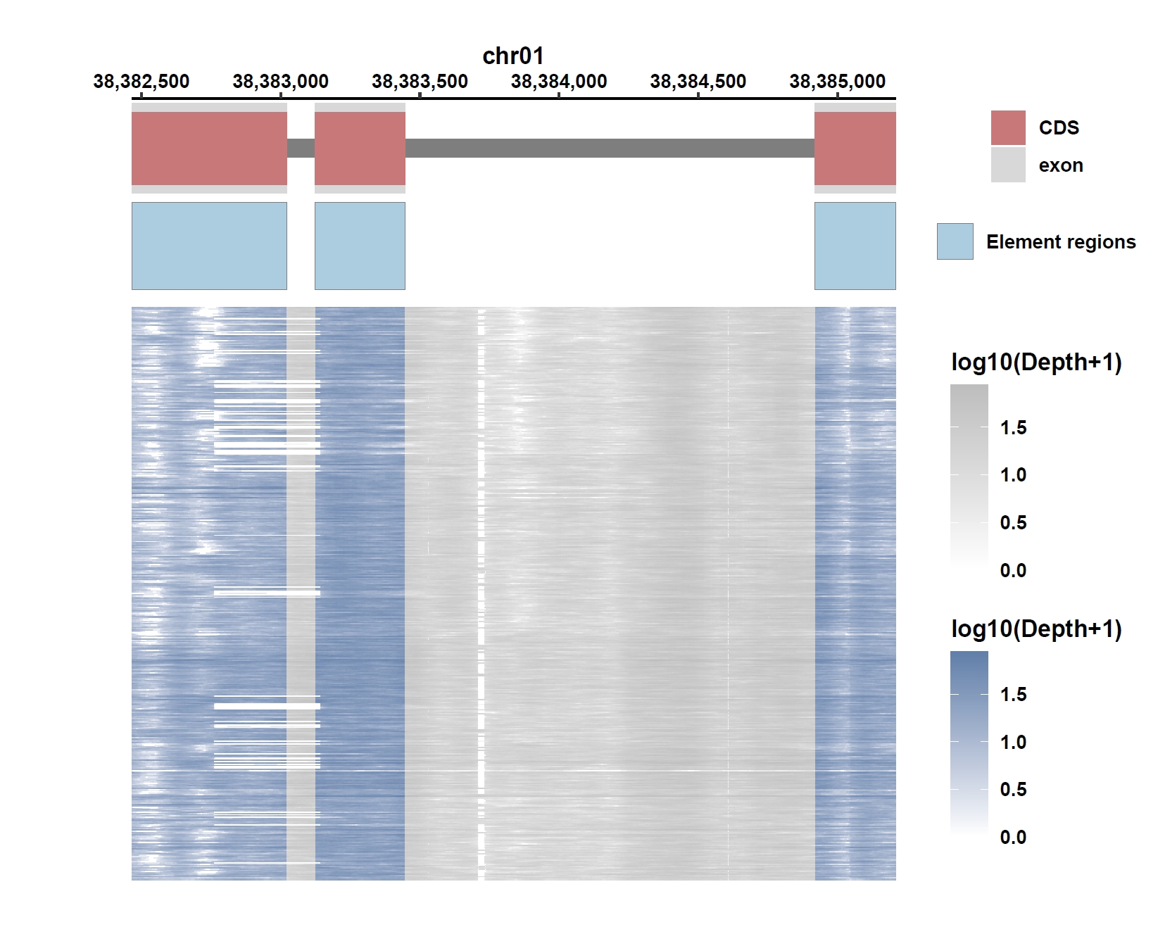
Plot coverage, PAV and depth:
apav elePlotCov --elecov Os01g0883800.elecov --gff Os01g0883800.gff  --hide_sample_name --top_anno_height 0.25 --fig_width 7.5 --fig_height 6
apav elePlotPAV --elepav Os01g0883800.elepav --gff Os01g0883800.gff --hide_sample_name --top_anno_height 0.25 --fig_width 7.5 --fig_height 6
apav elePlotDepth --ele Os01g0883800.elecov --bamdir ../data/rice_bam/ --gff Os01g0883800.gff --hide_sample_name --log10 --top_anno_height 0.25 --fig_width 7.5 --fig_height 6
Output: Os01g0883800.elecov.pdf, Os01g0883800.elepav.pdf, Os01g0883800.elecov.depth.pdf
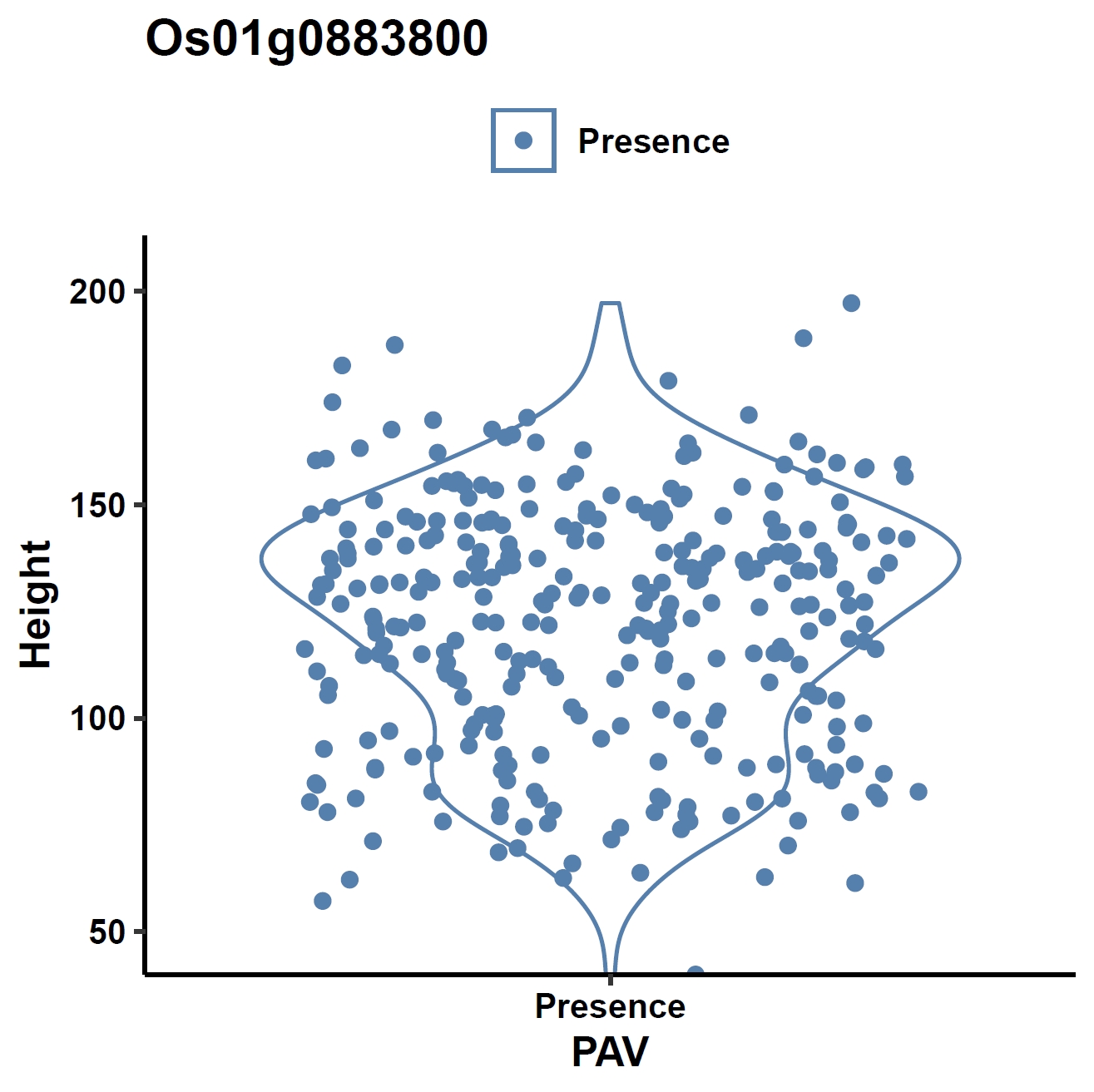
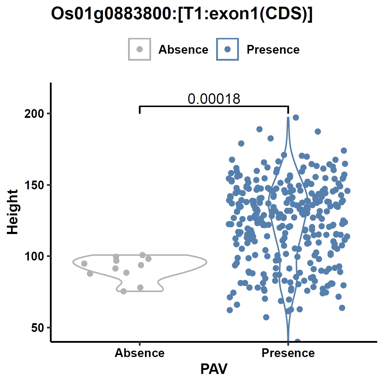
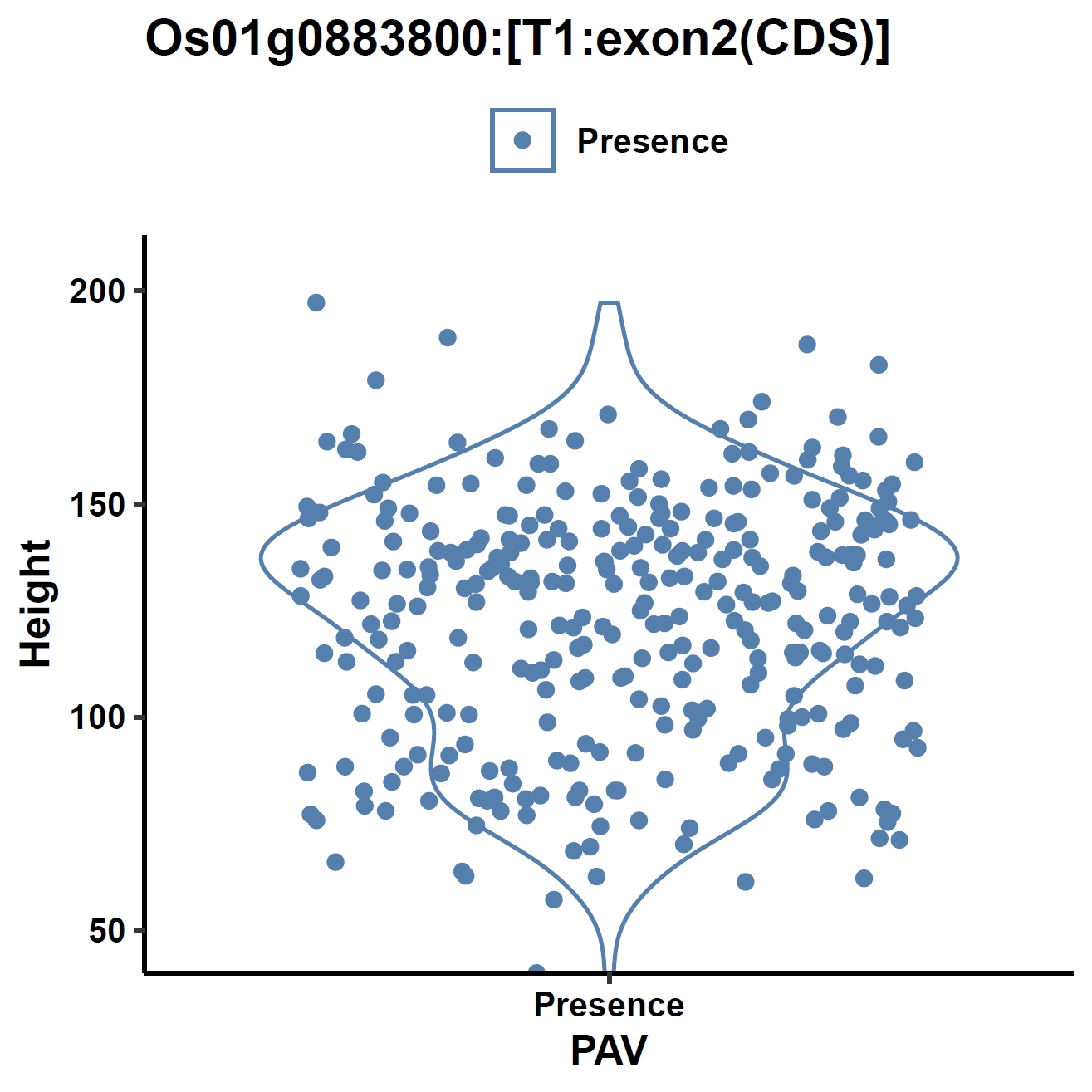
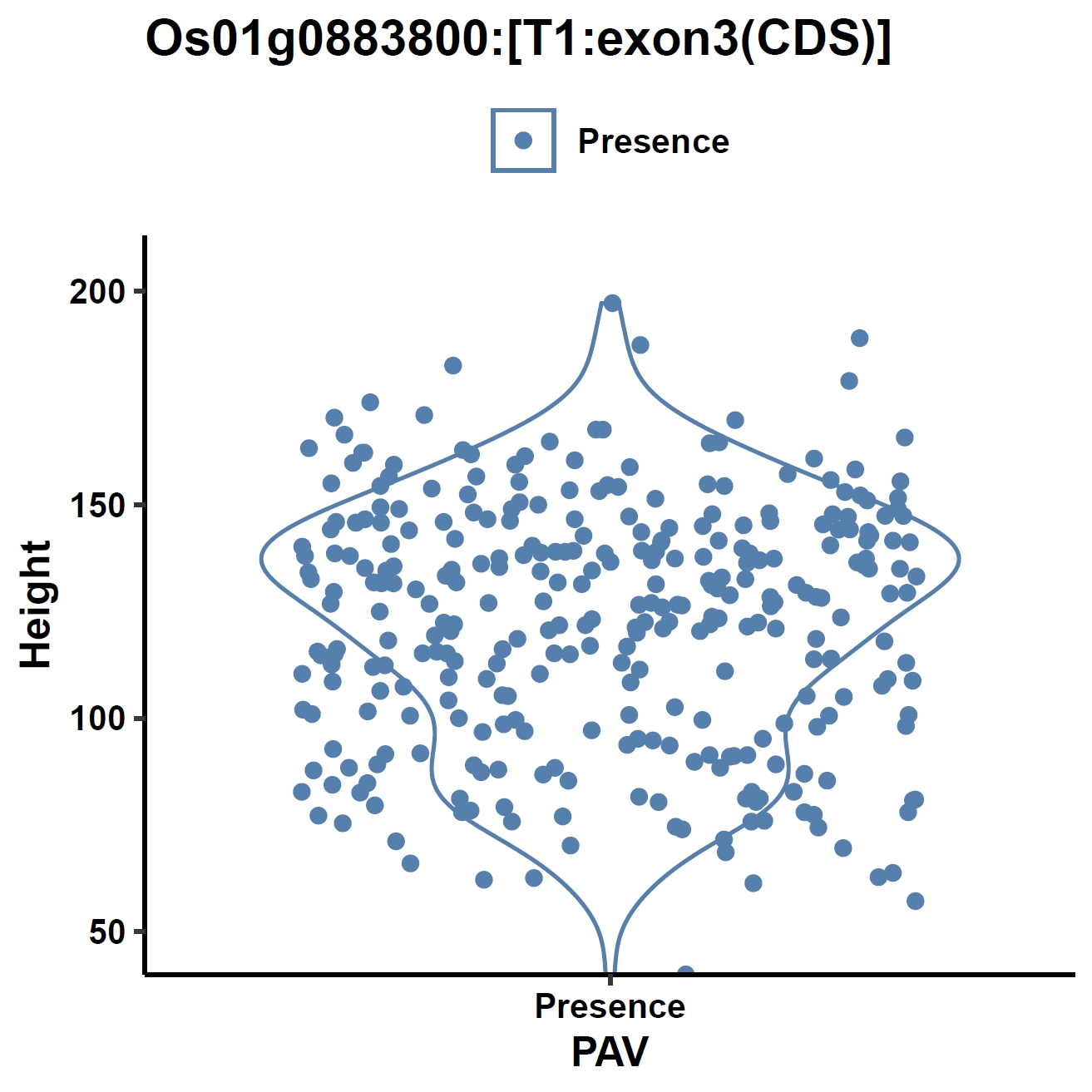
View phenotype association with plant height for gene and exons:
apav pavPlotPhenoVio --pav ../ricepan.pav --pheno ../data/rice.pheno --pheno_name Height --region_name Os01g0883800 --fig_width 4 --fig_height 4 --out Os01g0883800_height
apav pavPlotPhenoVio --pav Os01g0883800.elepav --pheno ../data/rice.pheno --pheno_name Height --region_name 'Os01g0883800:[T1:exon1(CDS)]' --fig_width 4 --fig_height 4 --out Os01g0883800_height_exon1
apav pavPlotPhenoVio --pav Os01g0883800.elepav --pheno ../data/rice.pheno --pheno_name Height --region_name 'Os01g0883800:[T1:exon2(CDS)]' --fig_width 4 --fig_height 4 --out Os01g0883800_height_exon2
apav pavPlotPhenoVio --pav Os01g0883800.elepav --pheno ../data/rice.pheno --pheno_name Height --region_name 'Os01g0883800:[T1:exon3(CDS)]' --fig_width 4 --fig_height 4 --out Os01g0883800_height_exon3
Output: Os01g0883800_height.pdf, Os01g0883800_height_exon1.pdf, Os01g0883800_height_exon2.pdf, Os01g0883800_height_exon3.pdf
Metrics
The computational experiments were performed on an x86-64 server equipped with dual Intel Xeon Gold 6248 processors.| Step | Input data | Run time |
|---|---|---|
| gff2bed | ricepan.gff(35M) | 5.0s |
| staCov | 453 BAM files and index files (5.44TB), ricepan.bed(15M) | 73h 5min (~9min 40s for one sample) |
| callPAV | ricepan.cov(75M) | 57.4s |
| callPAV | ricepan_ele.cov(180M) | 1min 29.2s |
| pavSize | ricepan.pav(48M) | 2min 1.5s |
| pavPlotSize | rice_grouped.size(1.1M) | 20.9s |
| pavPlotHist | ricepan.pav(48M) | 11.9s |
| pavPlotStat | ricepan.pav(48M) | 11.6s |
| pavPlotHeat | ricepan_dis.pav(22M) | 67.1s |
| pavPCA | ricepan_dis.pav(22M) | 10.8s |
| pavStaPheno | ricepan_dis.pav(22M), rice.pheno(13K) | 2min 33.3s |
| pavPlotPhenoMan | ricepan_dis.phenores(3.6M) | 9.4s |
| pavPlotPhenoVio | ricepan.pav(48M), rice.pheno(13K) | 11.6s |
| pavPlotPhenoBar | ricepan.pav(48M), rice.pheno(13K) | 11.5s |
| elePlotCov, elePlotPAV, elePlotDepth | Os04g0373400.elecov(16K), Os04g0373400.elepav(14K) | 5.6s, 5.6s, 1min 22.5s |
| pavPlotPhenoBar | Os04g0373400.elepav(14K), rice.pheno(13K) | 11.5s, 4.9s, 4.9s, 4.9s |
| elePlotCov, elePlotPAV, elePlotDepth | Os01g0883800.elecov(9.9K), Os01g0883800.elepav(8.4K) | 5.3s, 5.3s, 42.7s |
| pavPlotPhenoVio | Os01g0883800.elepav(8.4K), rice.pheno(13K) | 12.0s, 5.0s, 5.0s, 5.0s |
Gastric tumor
Code and Result
1. Coordinate Extraction
Extract genomic coordinates for genes, genetic elements, and flanking regions (1,000 bp upstream/downstream partitioned into 10 × 100 bp intervals) from GFF annotation files:apav gff2bed --gff data/gcpan.gff3 --chrl data/gcpan.chrl --up_n 10 --up_bin 100 --down_n 10 --down_bin 100
2. Coverage Calculation
Calculate coverage for gene and element regions across all samples based on alignment results, using the transcript with the longest CDS region as the representative transcript for the gene:apav staCov --bed gcpan.bed --bamdir data/gc_bam --asgene --rep cdslen ## This step will consume a lot of time and you can download the results directly: wget https://cgm.sjtu.edu.cn/APAV/case/gc/gcpan.cov && wget https://cgm.sjtu.edu.cn/APAV/case/gc/gcpan_ele.cov
3. PAV Determination
Determine gene PAV at 80% threshold (genes with coverage ≥80% are classified as "presence", otherwise "absence"):apav callPAV --cov gcpan.cov --pheno data/gc.pheno --thre 0.8
Determine element PAV at 80% threshold:
apav callPAV --cov gcpan_ele.cov --pheno data/gc.pheno --thre 0.8
4. Pangenome Size Estimation
Extract grouping information from the phenotype file:cat data/gc.pheno | cut -f 1,3 > gc.group apav pavSize --pav gcpan_all.pav --group gc.group --out gcpan_grouped.size
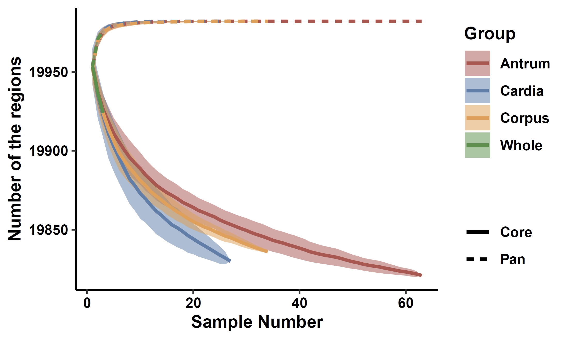
apav pavPlotSize --size gcpan_grouped.size --fig_height 3 --fig_width 5
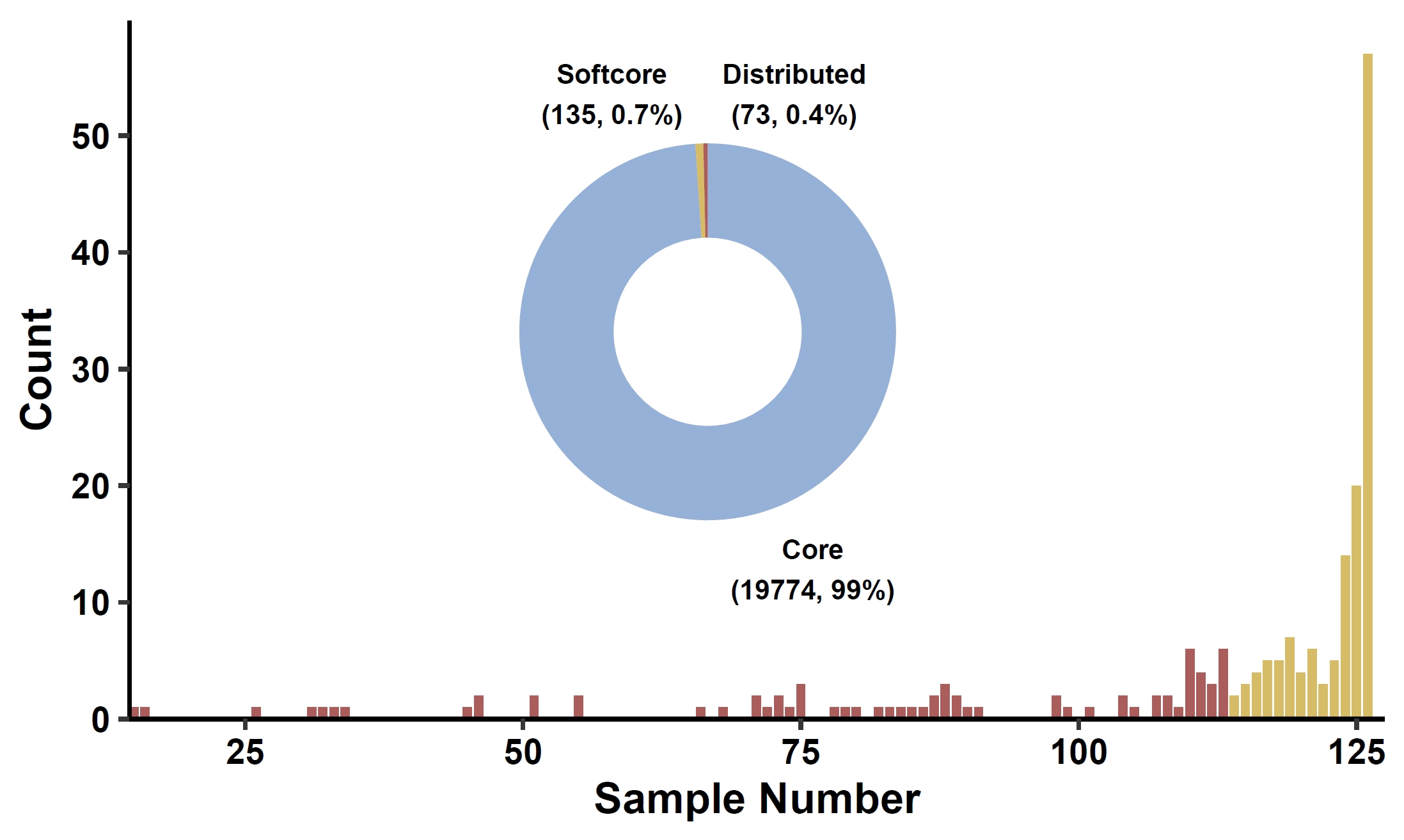
5. PAV analysis
Classify genes into core, soft-core, distributed, and private categories:apav pavPlotHist --pav gcpan_all.pav --ring_r 0.45 --ring_label_size 2.5 --fig_height 3 --fig_width 5
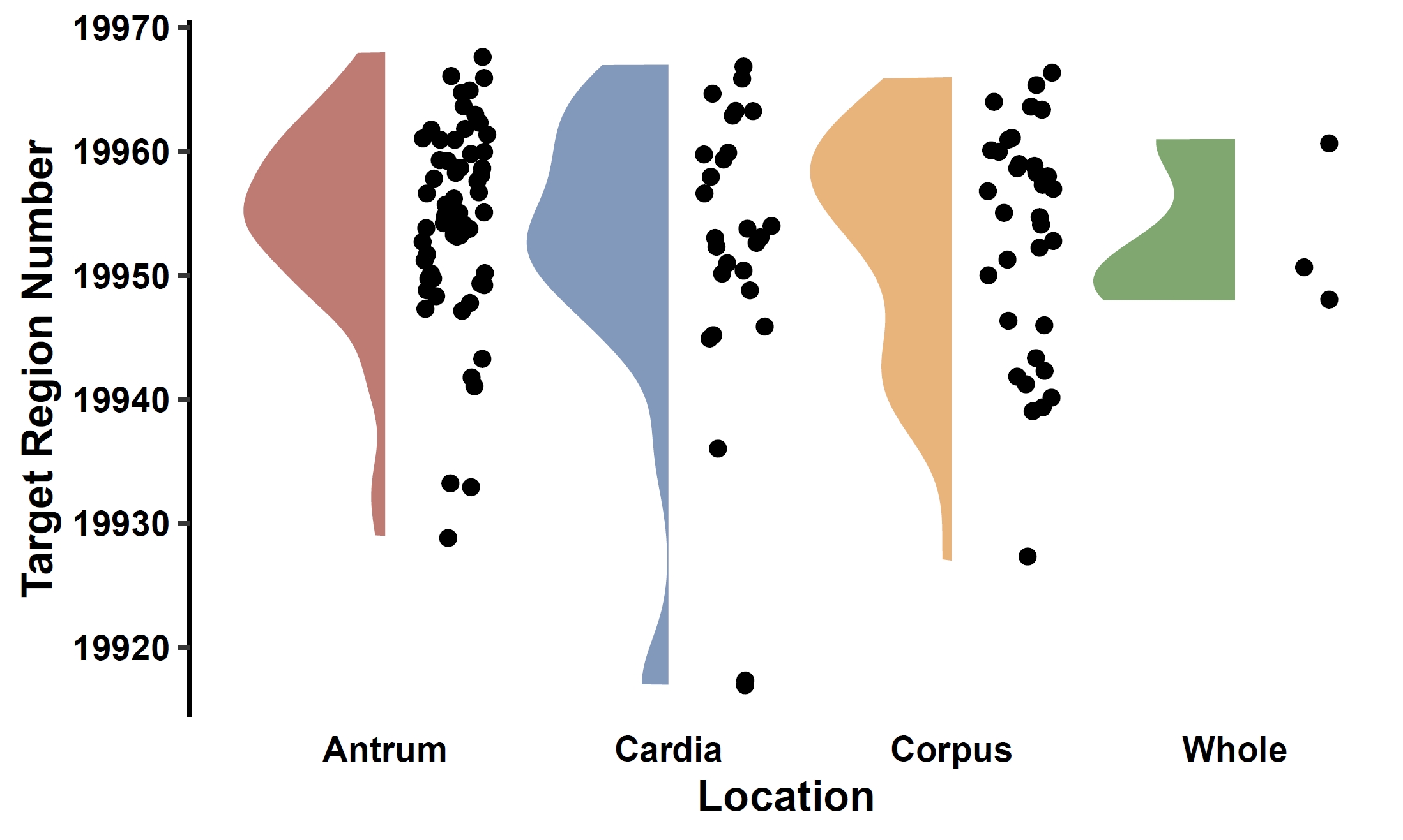
Compare gene counts across phenotype groups:
apav pavPlotStat --pav gcpan_all.pav --pheno data/gc.pheno --add_pheno_info Location --fig_width 5 --fig_height 3
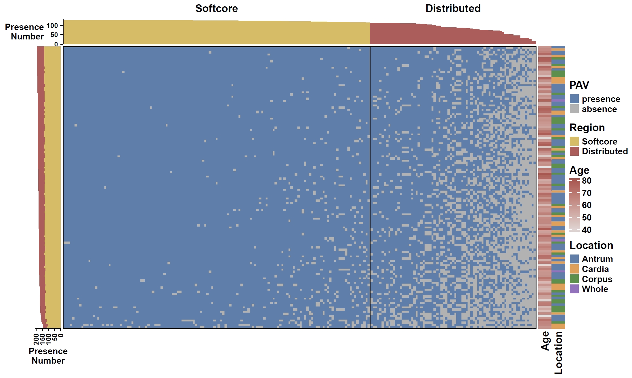
Plot heatmap for non-core genes:
cat data/gc.pheno | cut -f 1,2,3 > gc.anno
apav pavPlotHeat --pav gcpan_dispensable.pav --pheno gc.anno --anno_param_row_pheno name_side=bottom --fig_width 10 --fig_height 6
6. Phenotype Association Analysis
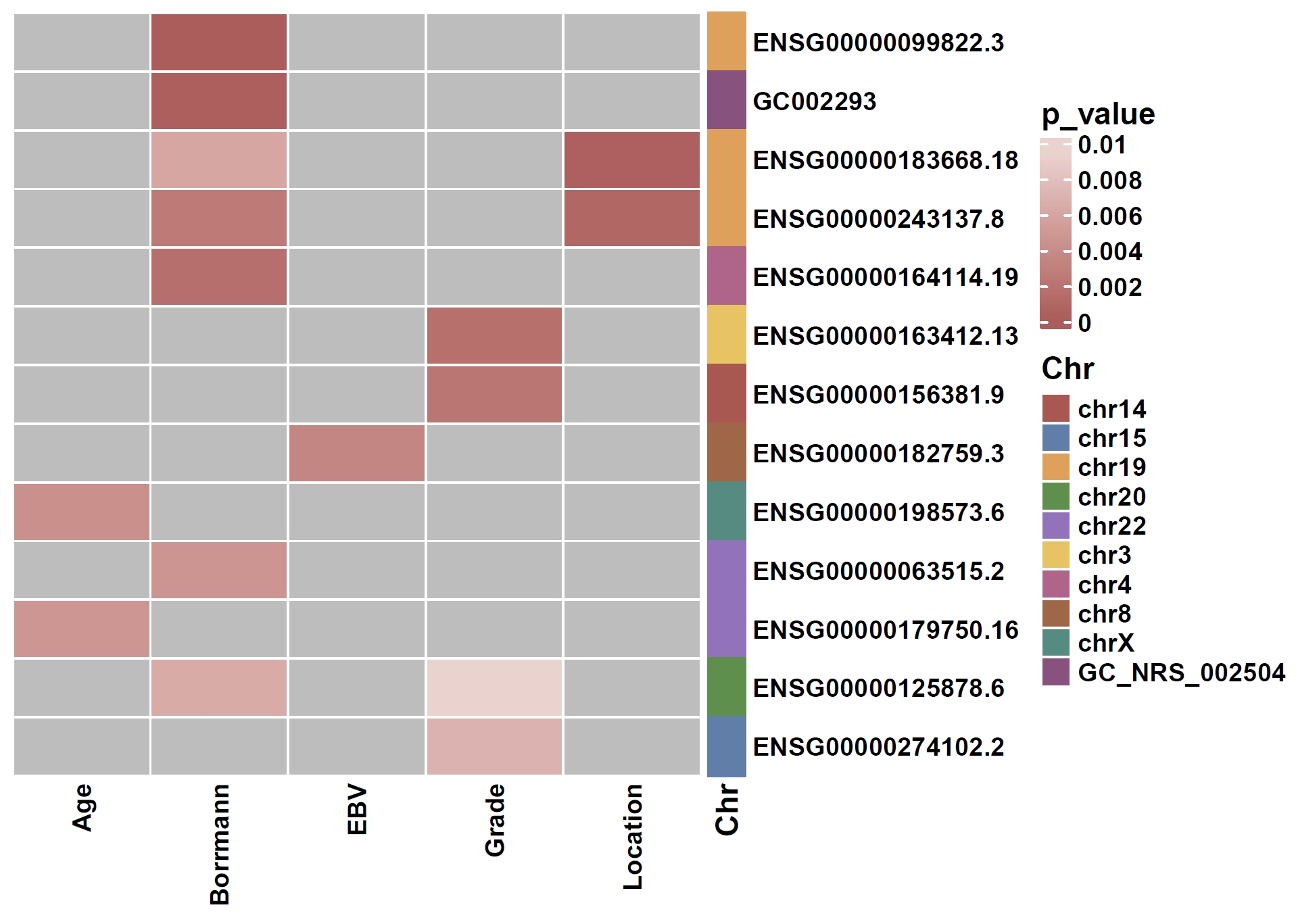
Calculate associations between non-core genes and phenotypes:apav pavStaPheno --pav gcpan_dispensable.pav --pheno data/gc.pheno
apav pavPlotPhenoHeat --pav gcpan_dispensable.pav --pheno data/gc.pheno --pheno_res gcpan_dispensable.phenores --only_show_significant --fig_height 5 --fig_width 7
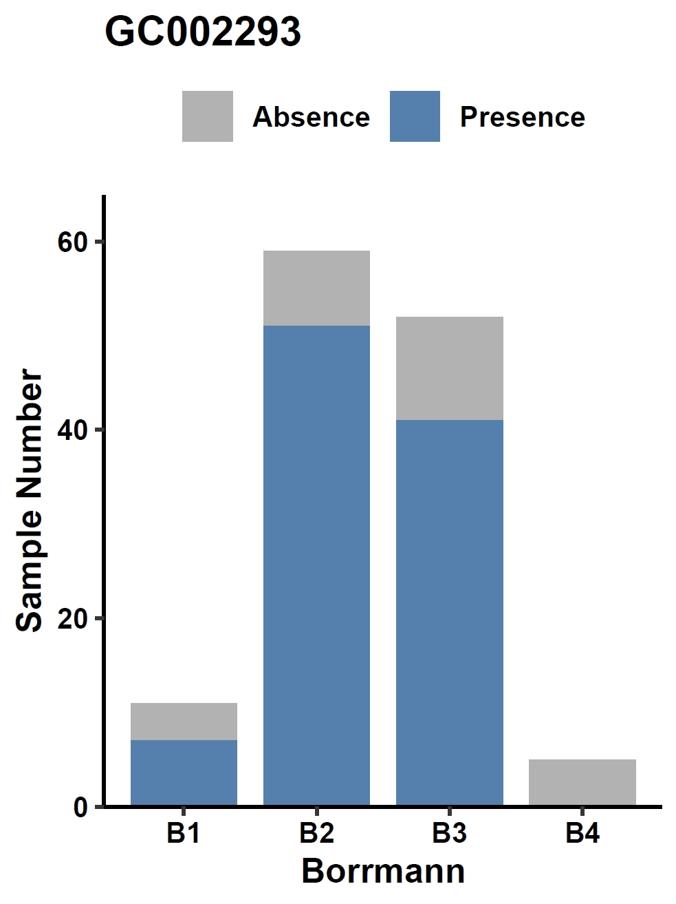
Visualize the association between a gene and a discrete phenotype (e.g., the GC002293 gene and Borrmann classification) in a bar plot:
apav pavPlotPhenoBar --pav gcpan_all.pav --pheno data/gc.pheno --pheno_name Borrmann --region_name GC002293 --fig_height 4 --fig_width 3
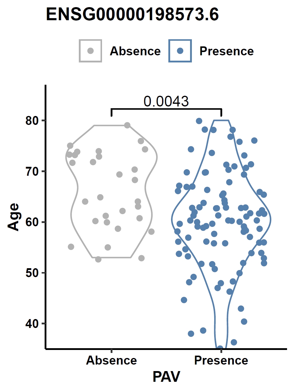
Visualize the association between gene PAV and a continuous phenotype (e.g., the ENSG00000198573.6 gene and age) in a violin plot:
apav pavPlotPhenoVio --pav gcpan_all.pav --pheno data/gc.pheno --pheno_name Age --region_name ENSG00000198573.6 --fig_height 4 --fig_width 3
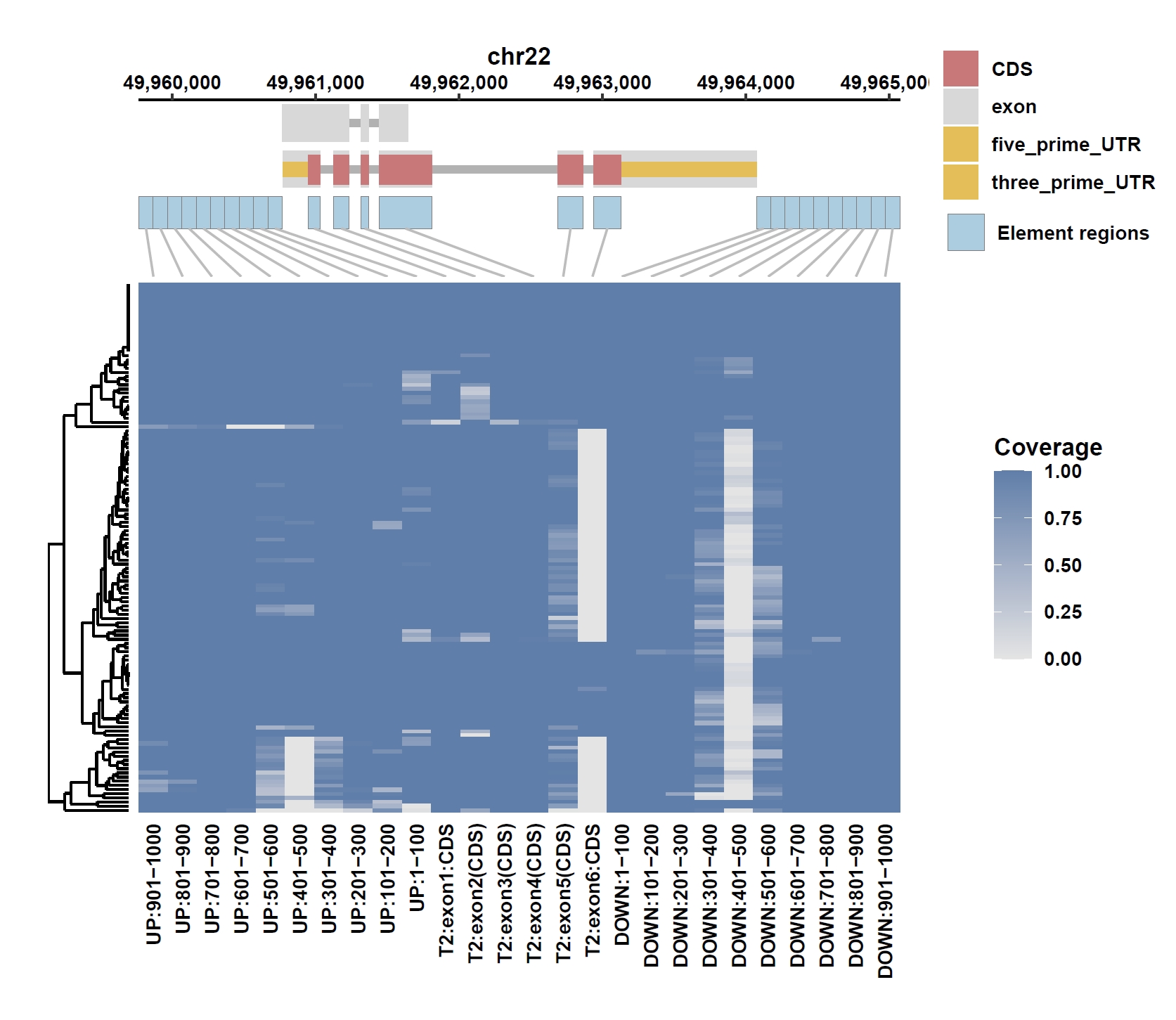
7. Element Visualization (ACOT1)
Prepare annotation and data files:mkdir ele_example_acot1 && cd ele_example_acot1 grep 'ENSG00000184227.8' ../data/gcpan.gff3 > ENSG00000184227.8.gff grep -E 'Annotation|ENSG00000184227.8' ../gcpan_ele.cov > ENSG00000184227.8.elecov grep -E 'Annotation|ENSG00000184227.8' ../gcpan_ele_all.pav > ENSG00000184227.8.elepav
Plot coverage, PAV and depth:
apav elePlotCov --elecov ENSG00000184227.8.elecov --gff ENSG00000184227.8.gff --cluster_samples --hide_sample_name --top_anno_height 0.25 --fig_width 7.5 --fig_height 6.5
apav elePlotPAV --elepav ENSG00000184227.8.elepav --gff ENSG00000184227.8.gff --cluster_samples --hide_sample_name --top_anno_height 0.25 --fig_width 7.5 --fig_height 6.5
apav elePlotDepth --ele ENSG00000184227.8.elecov --bamdir ../data/gc_bam/ --gff ENSG00000184227.8.gff --cluster_samples --hide_sample_name --log10 --top_anno_height 0.25 --fig_width 7.5 --fig_height 5.5
cd ..
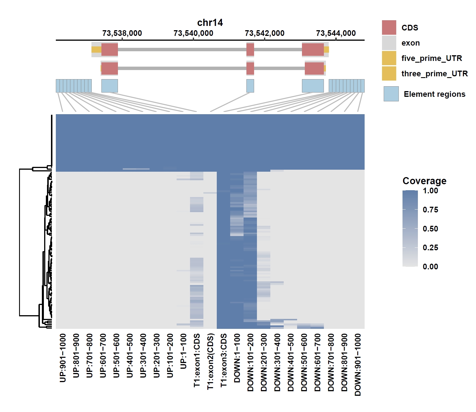
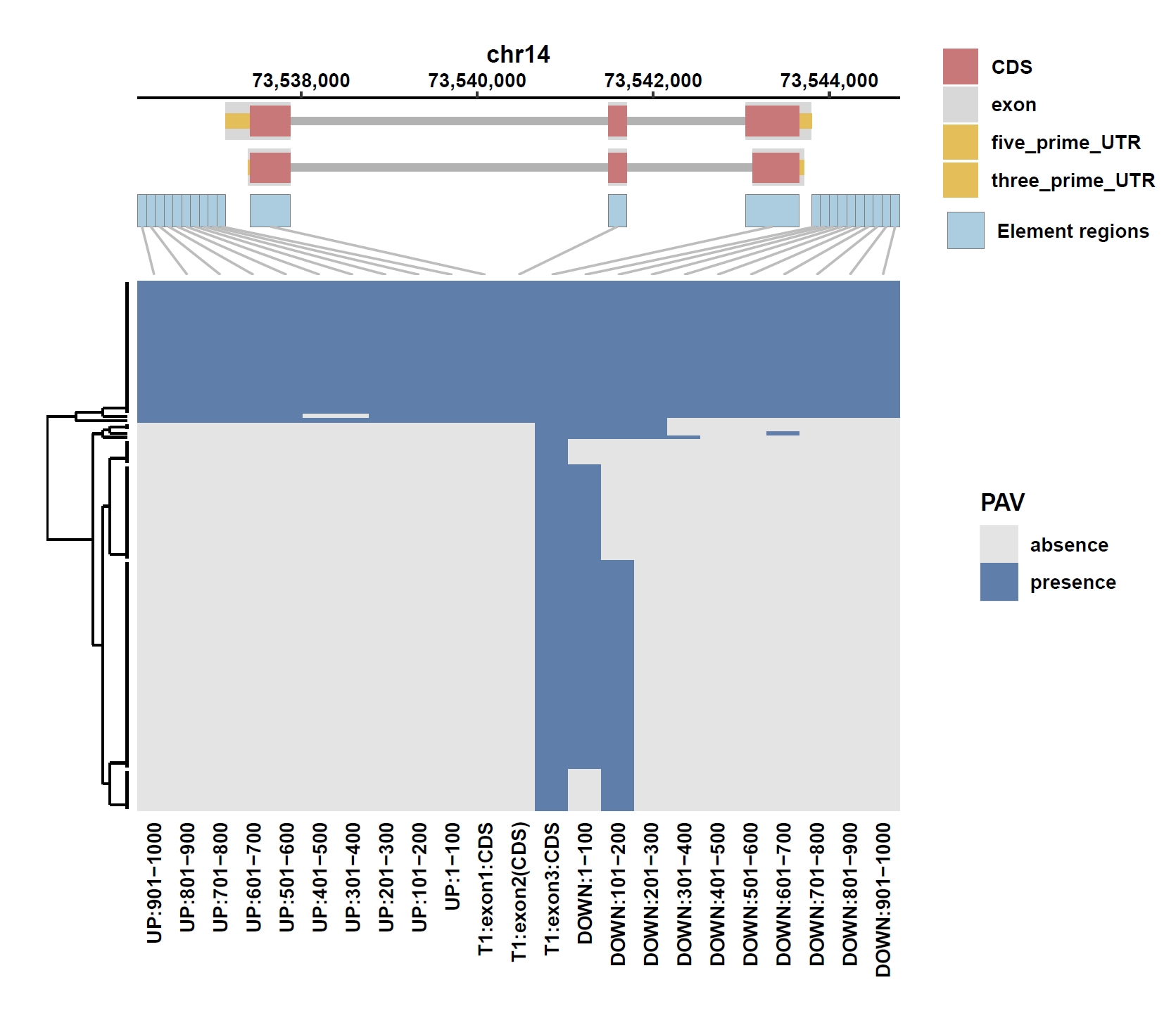
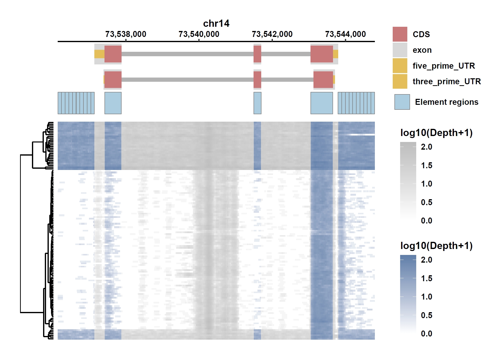
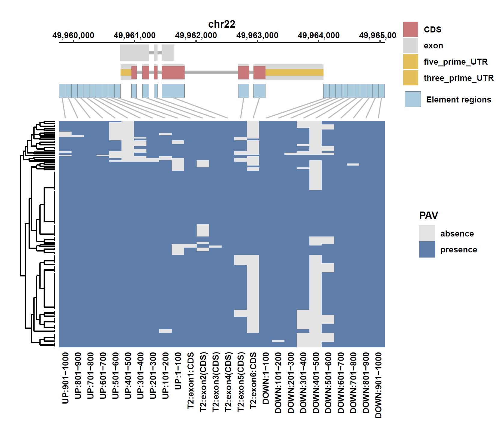
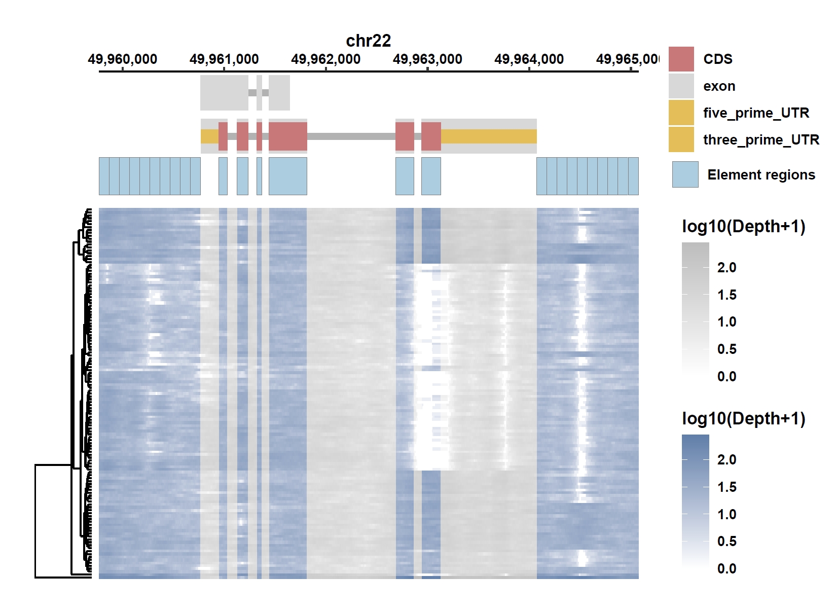
8. Element Visualization (PIM3)
Prepare annotation and data files:mkdir ele_example_pim3 && cd ele_example_pim3 grep 'ENSG00000198355.5' ../data/gcpan.gff3 > ENSG00000198355.5.gff grep -E 'Annotation|ENSG00000198355.5' ../gcpan_ele.cov > ENSG00000198355.5.elecov grep -E 'Annotation|ENSG00000198355.5' ../gcpan_ele_all.pav > ENSG00000198355.5.elepav
Plot coverage, PAV and depth:
apav elePlotCov --elecov ENSG00000198355.5.elecov --gff ENSG00000198355.5.gff --cluster_samples --hide_sample_name --top_anno_height 0.25 --fig_width 7.5 --fig_height 6.5
apav elePlotPAV --elepav ENSG00000198355.5.elepav --gff ENSG00000198355.5.gff --cluster_samples --hide_sample_name --top_anno_height 0.25 --fig_width 7.5 --fig_height 6.5
apav elePlotDepth --ele ENSG00000198355.5.elecov --bamdir ../data/gc_bam/ --gff ENSG00000198355.5.gff --cluster_samples --hide_sample_name --log10 --top_anno_height 0.25 --fig_width 7.5 --fig_height 5.5
Output: ENSG00000198355.5.elecov.pdf, ENSG00000198355.5.elepav.pdf, ENSG00000198355.5.elecov.depth.pdf
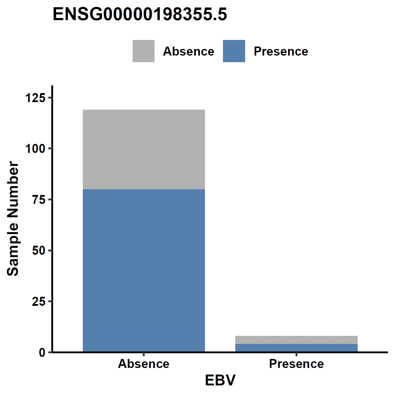
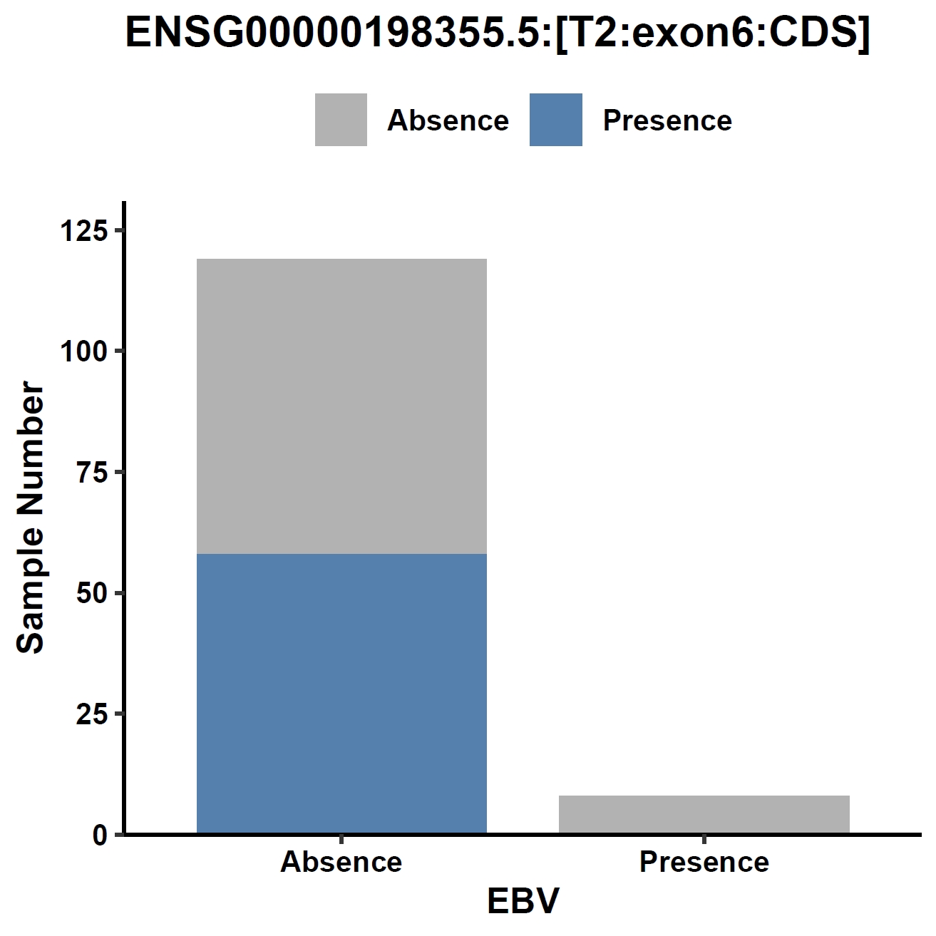
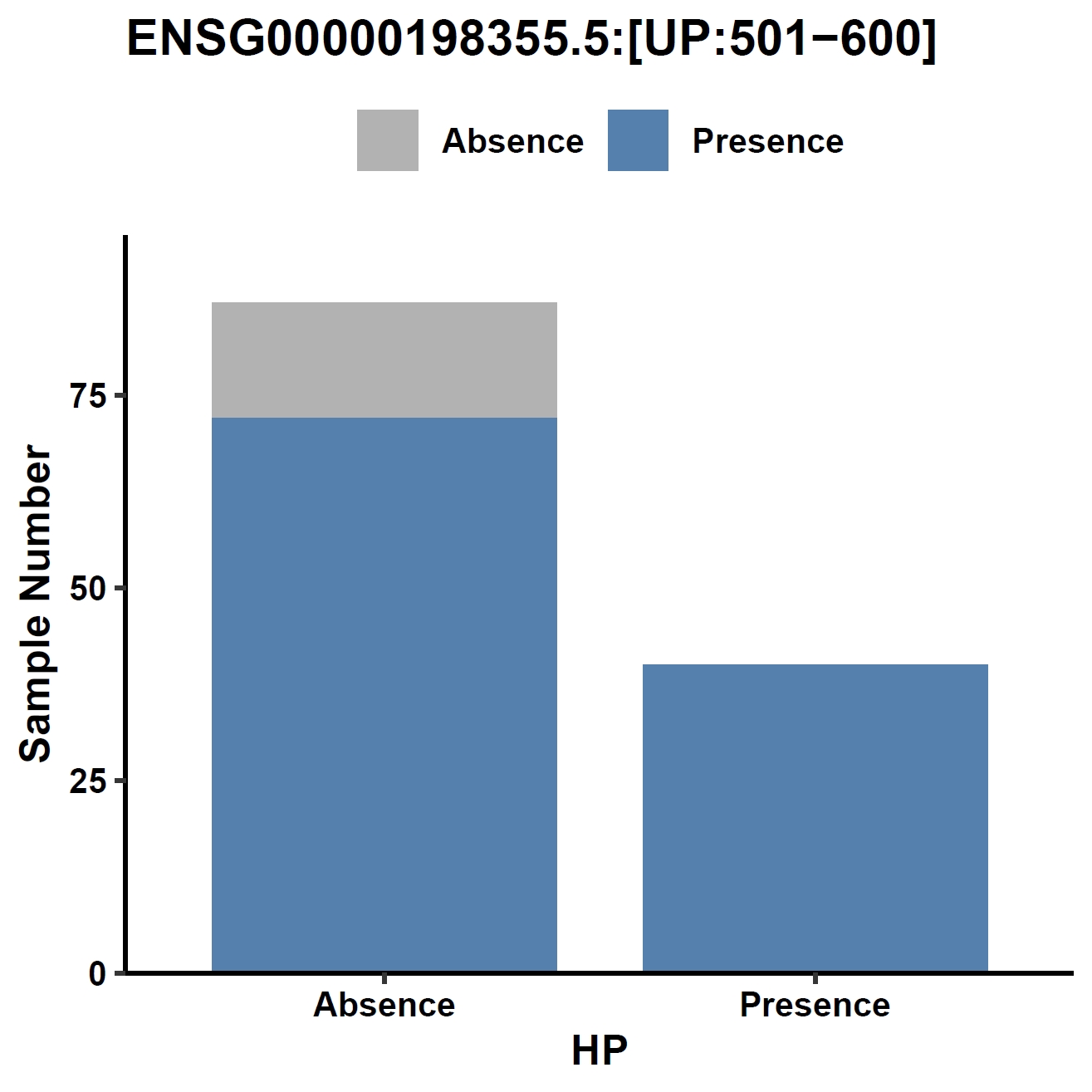
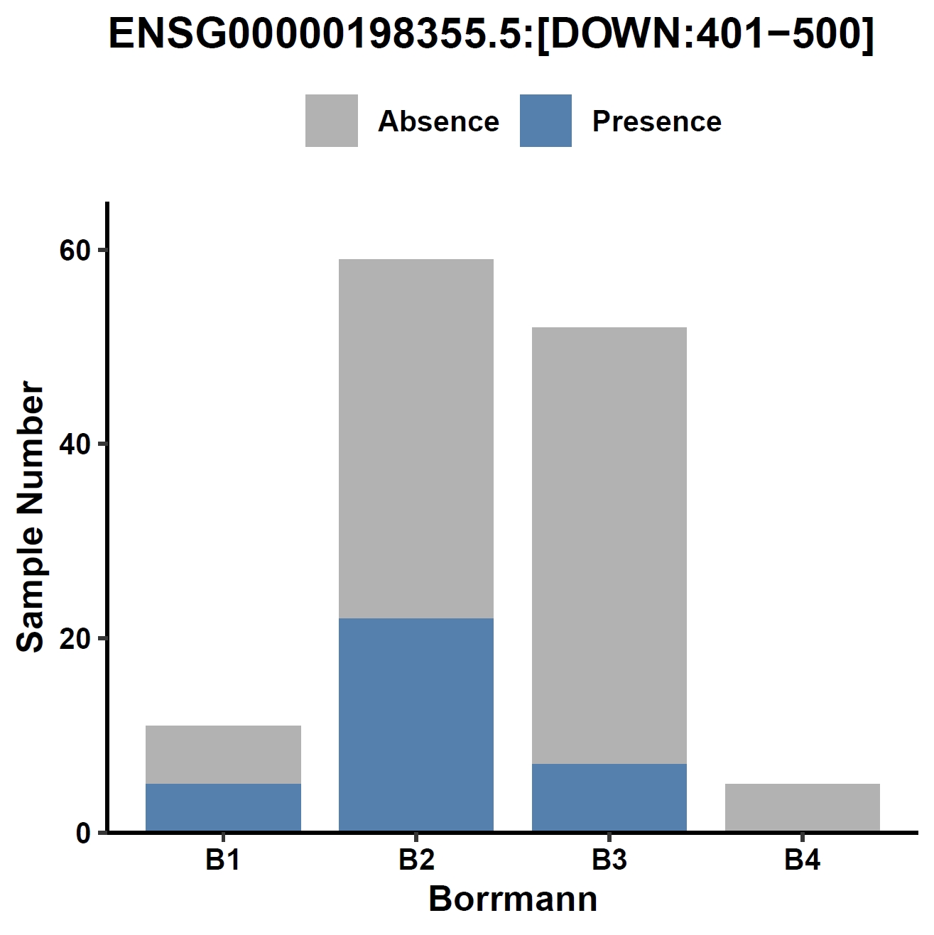
View phenotype association with phenotypes for gene and exons:
apav pavPlotPhenoBar --pav ../gcpan_all.pav --pheno ../data/gc.pheno --pheno_name EBV --region_name ENSG00000198355.5 --fig_width 4 --fig_height 4 --out ENSG00000198355.5_ebv
apav pavPlotPhenoBar --pav ENSG00000198355.5.elepav --pheno ../data/gc.pheno --pheno_name EBV --region_name 'ENSG00000198355.5:[T2:exon6:CDS]' --fig_width 4 --fig_height 4 --out ENSG00000198355.5_ebv_exon6
apav pavPlotPhenoBar --pav ENSG00000198355.5.elepav --pheno ../data/gc.pheno --pheno_name HP --region_name 'ENSG00000198355.5:[UP:501-600]' --fig_width 4 --fig_height 4 --out ENSG00000198355.5_hp_up
apav pavPlotPhenoBar --pav ENSG00000198355.5.elepav --pheno ../data/gc.pheno --pheno_name Borrmann --region_name 'ENSG00000198355.5:[DOWN:401-500]' --fig_width 4 --fig_height 4 --out ENSG00000198355.5_borrmann_down
cd ..
Output: ENSG00000198355.5_ebv.pdf, ENSG00000198355.5_ebv_exon6.pdf, ENSG00000198355.5_hp_up.pdf, ENSG00000198355.5_borrmann_down.pdf
Metrics
The computational experiments were performed on an x86-64 server equipped with dual Intel Xeon Gold 6248 processors.| Step | Input data | Run time |
|---|---|---|
| gff2bed | gcpan.gff3(1.2G) | 21.6s |
| staCov | 127 BAM files and index files (11.94TB), gcpan.bed(113M) | 120h 7min (~1h 9min for one sample) |
| callPAV | gcpan.cov(9.1M) | 2.9s |
| callPAV | gcpan_ele.cov(181M) | 40.0s |
| pavSize | gcpan_all.pav(8.9M) | 1.9s |
| pavPlotSize | gcpan_grouped.size(331K) | 5.0s |
| pavPlotHist | gcpan_all.pav(8.9M) | 6.0s |
| pavPlotStat | gcpan_all.pav(8.9M) | 5.7s |
| pavPlotHeat | gcpan_dispensable.pav(76K) | 8.6s |
| pavStaPheno | gcpan_dispensable.pav(76K), gc.pheno(4.3K) | 5.3s |
| pavPlotPhenoHeat | gcpan_dispensable.phenores(54K) | 5.0s |
| pavPlotPhenoBar | gcpan_all.pav(8.9M), gc.pheno(4.3K) | 5.7s |
| pavPlotPhenoVio | gcpan_all.pav(8.9M), gc.pheno(4.3K) | 5.9s |
| elePlotCov, elePlotPAV, elePlotDepth | ENSG00000184227.8.elecov(9.2K), ENSG00000184227.8.elepav(8.4K) | 5.5s, 5.4s, 25.1s |
| elePlotCov, elePlotPAV, elePlotDepth | ENSG00000198355.5.elecov(11K), ENSG00000198355.5.elepav(9.3K) | 5.5s, 5.4s, 22.5s |