Integrated command
The process can be automated with the “geneBatch” or “generalBatch” command, which entails extracting coordinates, computing coverage, identifying PAVs, and generating web reports, along with default preview figures. Users can also use APAV's visualization commands in a Linux environment or the APAVplot R package in R for enhanced visualization.
After running the command, you will get the following results:
| A file with the suffix ".bed" | Coordinates of genetic elements. (only for the "geneBatch" command) | |
| The files with the suffix ".cov" and "_ele.cov" | Coverage profile of target region and element region. | |
| A file with the suffix "_ele.mcov" | Coverage profile of merged element region. (with the "--merge" option) | |
| The files with the suffix "_all.pav" and "_ele_all.pav" | PAV profile of target region and element region. | |
| The files with the suffix "_dispensable.pav" and "_ele_dispensable.pav" | PAV profile of dispensable region. | |
| A file with the suffix ".fpav" | PAV profile of gene family. (only for the "geneBatch" command with the "--fam" option) | |
| A folder with the suffix "_report" | A file named "PAV" | A web report for PAV profile. |
| A file named "Sample" | A web report for samples. | |
| A folder named "js" | JS files. | |
| A folder named "css" | CSS files. | |
| A folder named "browser" | Data for tracks in the genome browser. | |
| A folder with the suffix "_ele_report" | A file named "PAV" | An interactive web report for PAV profile. |
| A file named "Sample" | An interactive web report for samples. | |
| A folder named "js" | JS files. | |
| A folder named "css" | CSS files. | |
| A folder named "estimation" | A file with the suffix ".size" | The result of estimation. |
| A PDF file with the suffix "_size_curve" | The growth curve of genome estimation. | |
| A folder named "coverage_visualization" | A PDF file with the suffix "_cov_heatmap" | A heatmap of coverage profile. |
| A folder named "common_analysis" | A PDF file with the suffix "_all_pav_sta" | A half-violin chart to show the number of regions. |
| A PDF file with the suffix "_all_pav_hist" | A ring chart and a histogram to show the classifications and distribution of target regions. | |
| A PDF file with the suffix "_all_pav_stackbar" | A stacked bar chart to show the classifications of target regions in all samples. | |
| A PDF file with the suffix "_dispensable_pav_cluster" | A circular clustering tree for the samples. | |
| A PDF file with the suffix "_dispensable_pav_pca" | A scatter plot presenting the results of the PCA analysis | |
| A folder named "phenotype_association" | A file with the suffix ".phenores" | The result of phenotype association. |
| The PDF files with the suffix "_manhattan" | Manhattan plots for phenotypes. | |
| The PDF files with the suffix "_block" | The chart drawn by "pavPlotPhenoBlock" command for discrete phenotypes. | |
| A folder named "example" | Some examples to show the effect of commands "pavPlotPhenoBar" and "pavPlotPhenoVio". | |
| A folder named "element_visualization" | Some examples to show the effect of commands "elePlotCov", "elePlotPAV", and "elePlotDepth". | |
Coordinate extraction
When working with simple annotated target regions on the genome, you can use the BED file directly and skip this step. However, in most cases, the target region of interest is the gene, which is a complex annotated structure within the genome. The gff2bed command is used to extract the coordinates of genes and genetic elements from a GFF format file and then outputs them to a BED file for subsequent steps
Genetic elements with the same coordinates will be consolidated to remove redundancy:
- If an exon contains only CDS or UTR, it is labeled as "[exonN(CDS)]", "[exonN(3UTR)]" or "[exonN(5UTR)]".
- If an exon contains multiple components, it is described as "[exonN:CDS]", "[exonN:3UTR]" or "[exonN:5UTR]".
- If an exon is present in more than one transcript, the information is combined into "[TN:exonN:CDS,TN:exonN:CDS]".
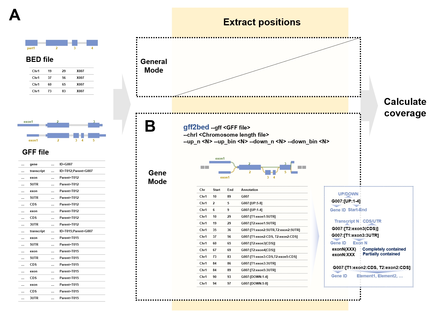
Schematic diagram of the gff2bed command. (A) Examples of input file formats. The BED file is used for arbitrary regions in general mode. The GFF file records annotation information for genes. (B) Overview of the parameters for the gff2bed command, along with the output generated from the example data. The diagonal line in the figure indicates that this step is skipped in the general mod. The blue dashed box shows the format of the gene element annotations. These annotations consist of two parts: the gene ID and the element list. Elements in the list are separated by commas, with each element detailing the transcript number, exon number, and the respective CDS or UTR category. Colons in the element annotations signify inclusion relationships, while parentheses indicate full inclusion.
Examples:
##Extracting the exon, CDS and UTR
$ apav gff2bed --gff demo1_gene.gff3
## Output: demo1_gene.bed
## Adding elements in upstream and downstream
$ apav gff2bed --gff demo1_gene.gff3 --chrl demo1.chrl \
  --up_n 10 --up_bin 100 --down_n 10 --down_bin 100
## Output: demo1_gene.bed
Coverage calculation
The staCov command is used to calculate the coverage of target regions and element regions by counting the percentage of covered bases. It calls samtools depth to compute the read depth at each position in the BAM files specified in the --bamdir parameter. A base is considered covered when the number of mapped reads exceeds the value specified in the --mincov parameter.
For genes, it offers six methods for selecting representative transcripts:
- "cdslen": using the transcript with the longest CDS region as the target region, and calculating coverage for the corresponding elements;
- "exonlen": using the transcript with the longest exon region as the target region, and calculating coverage of the corresponding elements;
- "len": using the longest transcript as the target region;
- "highcov": using the transcript with the highest coverage as the target region;
- "none": considering the entire gene body as the target region;
- "all": including all transcript regions, but calculating coverage only for the elements.
staCov command calculates both the coverage of the entire region and the coverage of the elements.
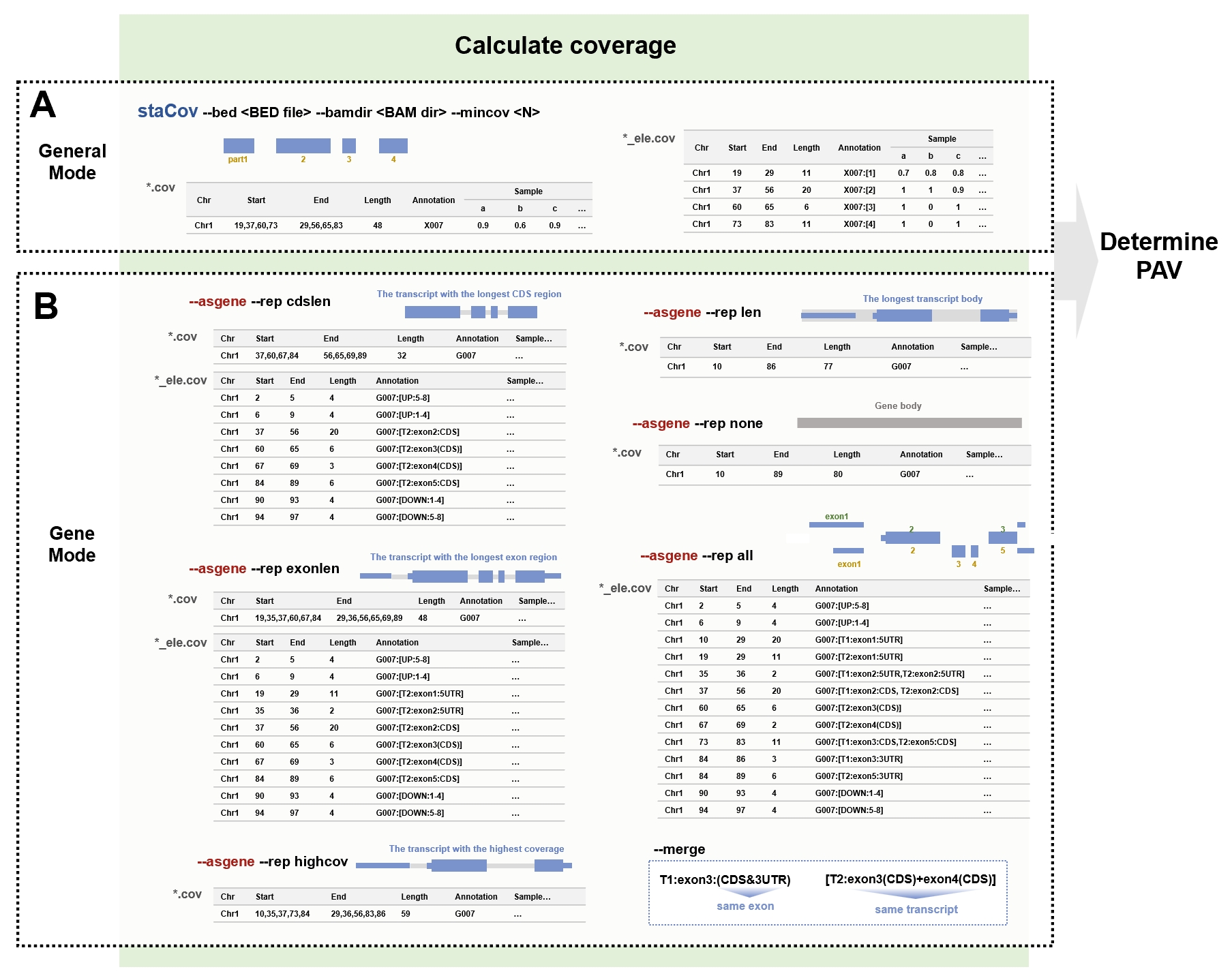
Description of the main parameters of the “staCov” command. (A) Key parameters in general mode. The user must provide the BED file and the directory containing the BAM file, and specify the coverage threshold (default value is 0.5). After running the command, two types of files will be generated. The file with suffixes “.cov” records the coverage of the whole region, while the file with suffixes “_ele.cov” specifically records the coverage of the elements. (B) Key parameters in gene mode. Similarly, the user must pass in the BED file (which can be generated using the gff2bed command), the directory containing the BAM file, and the coverage threshold (default value is also 0.5). Additionally, the --asgene parameter must be included to specify the target region to be treated as a gene. The --rep parameter allows for the selection of the region to be calculated. The “cdslen” option selects the transcript with the longest coding sequence (CDS) region, while “exonlen” selects the longest transcript in the exon region. The “highcov” option identifies the transcript with the highest coverage. The “len” option selects the longest transcript body, while ‘none’ indicates the selection of the gene body. The “all” option calculates the coverage of all elements without outputting the entire region.
Examples:
## Gene mode
$ apav staCov --bed demo1_gene.bed --bamdir bam --asgene --rep cdslen
## Output: demo1_gene.cov, demo1_gene_ele.cov
## General mode
$ apav staCov --bed demo2_general.bed --bamdir bam
## Output: demo2_general.cov, demo2_general_ele.cov
Additionally, the mergeEleCov command can merge neighboring regions with the same coverage (either all 0 or all 1). This sub-command is included within the staCov command and will be executed automatically when the --merge option is added.
For genes, the merged elements are symbolized as follows:
- When merging CDS and UTR on the same exon, they are represented as "exonN:(CDS&3UTR)" or "exonN:(CDS&5UTR)";
- When merging neighboring exons on the same transcript, they are represented as "exonN(CDS)+exonN(CDS)";
- When merging upstream or downstream elements, they are represented as "UP:N-N" or "DOWN:N-N".
Examples:
## Adding `--merge` option to `staCov` command
$ apav staCov --bed demo1_gene.bed --bamdir bam --asgene --merge --out demo1_m
## Ouput: demo1_m.cov, demo1_m_ele.cov, demo1_m_ele.mcov
## Using `mergeEleCov` command
$ apav mergeEleCov --elecov demo1_gene_ele.cov --asgene
## Output: demo1_gene_ele.mcov
The covPlotHeat visualization command provides an overview of coverage across samples in a complex heatmap. It calls R scripts and generates a PDF file. Users can display phenotype data alongside the heatmap using the --pheno option. The usage information and a complete parameter list can be obtained with apav covPlotHeat --help or apav covPlotHeat -h.
Examples:
$ apav covPlotHeat --cov demo1_gene.cov
## Default palette
$ apav covPlotHeat --cov demo1_gene.cov \
  --pheno demo_sample.pheno \
  --cluster_rows --cluster_columns \
  --show_row_names --row_names_side right
## Custom colors
$ apav covPlotHeat --cov demo1_gene.cov \
  --pheno demo_sample.pheno \
  --cluster_rows --cluster_columns \
  --show_row_names --row_names_side right \
  --cov_colors 'white,#D98D8D' \
  --pheno_info_color_list Location=#EDD12F,#C783C7 \
  --pheno_info_color_list Age=#C6E2FF,#6CA6CD
PAV determination
The callPAV command is used to determine presence or absence based on coverage. It offers two methods for PAV determination:
- Using a fixed threshold. Values greater than the threshold set by the
-tparameter are classified as present, while values below the threshold are classified as absent. - Using an adaptive threshold for each unit. If the sample with the highest uncovered percentage is smaller than the
-aparameter, all samples will be considered present. Otherwise, a clustering process is employed to identify the threshold. The clustering process involves the following steps:- Select the maximum and minimum values as the two centers of subgroups, then divide the other values into two groups based on their distance from the centers.
- Recalculate the median of each group to establish new centers.
- Regroup the values according to their distances from the new centers.
- Repeat the above steps until the grouping is stable (or the iteration count reaches the maximum threshold specified by the
-nparameter). Samples with smaller values are determined to be absent, while samples with larger values are determined to be present.
--fa, --gff, and --bamdir are optional and used to configure tracks in the genome browser. If these parameters are not added, the genome browser panel will not be included in the report. To include the genome browser panel, you must provide at least the --fa parameter, and the other two parameters can be provided as needed.
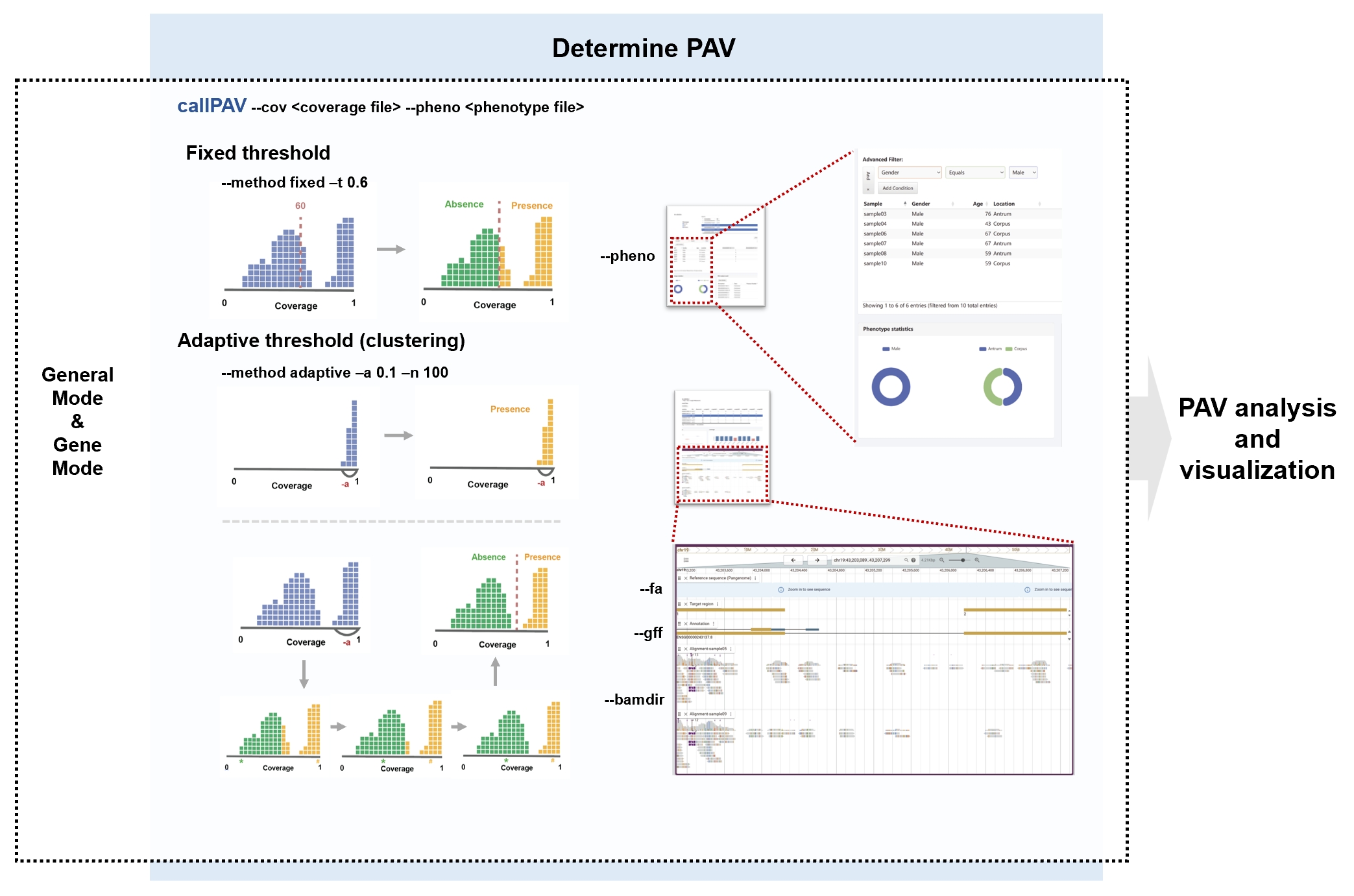
Description of the parameters of the callPAV command. The --cov parameter is used to input the coverage file. The --method parameter allows users to select the method for determining PAV. In the fixed threshold method, the -t parameter sets the coverage threshold: values above this threshold are classified as present, while those below are classified as absent. In the flexible threshold method, if none of the samples exceed the value specified by the -a parameter, all samples are classified as present. Otherwise, clustering is performed to differentiate between the presence and absence groups. The phenotype data specified by the --pheno parameter is used for the sample report. Data from the --fa, --gff and --bamdir parameters are displayed in the Genome Browser in the PAV report.
The final output includes PAV profiles and interactive web reports. PAV profiles contain all target regions and dispensable regions. In the PAV profile, 1 indicates presence, and 0 indicates absence. The reports are stored in a new folder that contains the PAV report, sample report, JS files, CSS files, and data files.
-
For the reports, please note the following points:
- You need to move the entire report folder (e.g.,
demo1_gene_report/) to the web server, maintaining the original file structure. Afterward, you can view the report by accessingPAV.htmlandsample.html. - Since BAM files are typically large, we provide two strategies to reduce storage space consumption. Under default settings, soft links will be created for BAM files and their index files to avoid redundant storage. If the
--sliceparameter is added, the target regions of interest will be extracted from the BAM files, thereby reducing the size of the BAM files. - If there are many dispensable regions, the
data.jsonfile may become excessively large, which could slowing web page loading. In such cases, you can group the results by dividing them by chromosomes or other methods to view the data more efficiently. - If you wish to download the results for local viewing, you must download the entire folder while preserving its structure. Due to the browser's Cross-Origin Resource Sharing (CORS) policy, the website may not display correctly because the data.json file cannot be accessed when you open the HTML file directly. We recommend using the web preview function of Dreamweaver to view the report.
The PAV report allows users to query and filter the PAV table. Users can click on the row for specific regions of interest to examine the coverage distribution for both the presence and absence groups. Additionally, users can view the values in a bar plot across all samples. There is also a sample table report that allows users to filter samples based on phenotypes and PAV results. For the filtered samples, users can examine the new PAV analysis result in real-time within a subpopulation.
Examples:
$ apav callPAV --cov demo1_gene.cov --pheno demo_sample.pheno --thre 0.5
## Output: demo1_gene_all.pav, demo1_gene_dispensable.pav, demo1_gene_report/

$ apav callPAV --cov demo1_gene_ele.cov --pheno demo_sample.pheno --thre 0.5
## Output: demo1_gene_ele_all.pav, demo1_gene_ele_dispensable.pav, demo1_gene_ele_report/
Here we show the document tree of the result:
demo/
├── demo1_gene_all.pav
├── demo1_gene_dispensable.pav
├── demo1_gene_reprot/
│   ├── css/
│   ├── js/
│   ├── data.json
│   ├── PAV.html
│   └── sample.html
├── demo1_gene_ele_all.pav
├── demo1_gene_ele_dispensable.pav
└── demo1_gene_ele_reprot/
    ├── css/
    ├── js/
    ├── data.json
    ├── PAV.html
    └── sample.html
Examples:
$ apav callPAV --cov demo1_gene.cov --pheno demo_sample.pheno --thre 0.5 \
  --fa demo.fa.gz --gff demo1_gene.gff3 --bamdir bam
## Output: demo1_gene_all.pav, demo1_gene_dispensable.pav, demo1_gene_report/
Here we show the tree of the report document:
demo1_gene_reprot
 ├── browser/
 │   ├── reference.fa.gz
 │   ├── reference.fa.gz.fai
 │   ├── reference.fa.gz.gzi
 │   ├── reference.gff.gz
 │   ├── reference.gff.gz.tbi
 │   ├── target.bb
 │   ├── sample01.bam
 │   ├── sample01.bam.bai
 │   └── ...
 ├── css/
 ├── js/
 ├── data.json
 ├── PAV.html
 └── sample.html
The reports of the demo data can be viewed in here.
After obtaining the PAV (Presence-Absence Variation) results for genes, you can further calculate the PAV for gene families. If at least one gene within a gene family is present, the gene family is marked as present; otherwise, it is marked as absent.
Examples:
$ apav gFamPAV --pav demo1_gene_all.pav --fam demo1_gene.fam
## Output: demo1_gene_all.gfpav
Genome estimation
The pavSize command is used to estimate the sizes of both the pangenome and core genome derived from the PAV table. The -n parameter sets the number of estimations. The estimation can be performed for all groups after adding the --group option.
Examples:
$ apav pavSize --pav demo1_gene_all.pav
## Output: demo1_gene_all.size
## Estimation in groups
$ cat demo_sample.pheno | cut -f 1,2 > demo_sample.group
$ apav pavSize --pav demo1_gene_all.pav --group demo_sample.group --out demo1_gene_all_group.size
## Output: demo1_gene_all_group.size
The pavPlotSize command utilizes the output table from pavSize to generate a growth curve illustrating the estimation of genome size. It calls R scripts and generates a PDF file. The --data_type option provides an identity count of the pangenome and core genome, or an increase of the pangenome. It offers three chart types: "errorbar", "jitter" and "ribbon" set by the --chart_type option. The usage information and parameter list can be obtained with apav pavPlotSize --help or apav pavPlotSize -h.
Examples:
$ apav pavPlotSize --size demo1_gene_all.size
$ apav pavPlotSize --size demo1_gene_all.size \
  --path_color '#e38e28,#298022' --ribbon_fill '#e38e28,#298022' --ribbon_alpha 0.2
$ apav pavPlotSize --size demo1_gene_all.size \
  --data_type increasing \
  --chart_type errorbar
$ apav pavPlotSize --size demo1_gene_all_group.size
PAV analysis and visualization
The target regions are categorized into core regions (present in all individuals) and dispensable regions (not present in all individuals). The dispensable regions can be further divided into softcore regions, distributed regions and private regions. Regions with loss rates that do not exceed the --softcore_loss_rate are classified as softcore regions. Regions that are found in only one sample are labeled as private regions, while all other regions are referred to as distributed regions. If adding the --use_binomial option, a binomial test is conducted (with a null hypothesis of loss rate < --softcore_loss_rate. A p-value below the --softcore_p_value option indicates that this target region is lost in a significant proportion, classifying it as a "distributed region" (with a loss rate > --softcore_loss_rate).
APAV offers a variety of visualization functions. The pavPlotStat command generates a half-violin plot to show the number of target regions present in samples. The pavPlotHist command combines a ring chart and a histogram to display the distribution of target regions. The pavPlotHeat command creates a heatmap along with two summary annotations. The pavPlotBar command allows users to view the composition of genes across all samples. The pavPCA command performs PCA analysis for PAV data, and the pavCluster command clusters samples based on the PAV table. The usage information and parameter list for each command can be shown with the --help or -h option after each command name.
pavPlotStat:
The number of target regions present in samples is shown in a half-violin plot. The left half represents the density estimate and each point on the right represents a sample.
## Example:
$ apav pavPlotStat --pav demo1_gene_all.pav --fig_width 4 --fig_height 3
$ apav pavPlotStat --pav demo1_gene_all.pav \
  --pheno demo_sample.pheno --add_pheno_info Location \
  --pheno_info_colors '#e38e28,#298022' \
  --fig_width 4 --fig_height 3
pavPlotHist:
The target regions can be categorized into different types based on the number of samples that contain them. The pavPlotHist command combines a ring chart and a histogram to display the distribution of target regions. The options --ring_pos_x, --ring_pos_y, and --ring_r are used to specify the position and radius of the ring chart. The x-axis of the histogram represents the number of samples, ranging from 1 to all samples, while the y-axis represents the number of regions shared by the specified number of samples.
## Example:
$ apav pavPlotHist --pav demo1_gene_all.pav --ring_pos_x 0.3 --ring_r 0.4
pavPlotHeat:
Heatmap is an intuitive way to display total PAV data. The pavPlotHeat command provides a heatmap and two summary annotations. The options --anno_param_row_stat and --anno_param_column_stat are used to set the parameters for the annotations. The columns can be split into blocks based on the classification of target regions. The names of blocks in the upper panel can be adjusted using the --block_name_size and --block_name_rot option.
The phenotype data can be displayed alongside the heatmap using the --pheno option. The --anno_param_row_pheno option controls the settings for phenotype annotations. The options --cluster_rows, --clustering_distance_rows, --clustering_method_rows, --cluster_columns, --clustering_distance_columns, --clustering_method_columns are used to cluster samples or regions. And the options --row_dend_side, --row_dend_width, --column_dend_side and --column_dend_height set the position and height of the dendrogram.
The --pav_volors option defines the colors for presence and absence. The --type_colors option defines the colors for classifications of the region.
## Example:
## Default palette
$ apav pavPlotHeat --pav demo1_gene_all.pav --pheno demo_sample.pheno \
  --block_name_rot 90 --fig_height 6 --fig_width 8

## Custom colors
$ apav pavPlotHeat --pav demo1_gene_all.pav --pheno demo_sample.pheno \
  --block_name_rot 90 --fig_height 6 --fig_width 8 \
  --pav_colors '#D98D8D,white' \
  --type_colors '#A4C9E3,#6CA6CD,#3E759C' \
  --pheno_info_color_list Gender=#e38e28,#E8D151
pavPlotBar:
The pavPlotBar command is used to view the composition of genes in all samples. The chart consists of a hierarchically clustered tree and a bar plot. The options --dend_width and --name_width determine the relative widths of the dendrogram and sample names. The dashed line and number labels indicate the mean value of cumulative sums when using the --show_relative option. Additionally, the --type_colors option allows you to define colors for region classifications, and you can customize colors for phenotypes using the --pheno_info_color_list option.
## Example:
$ apav pavPlotBar --pav demo1_gene_all.pav \
--pheno demo_sample.pheno --add_pheno_info Gender \
--fig_height 6 --fig_width 8
pavPCA:
The pavPCA command will perform PCA analysis for PAV data using the function prcomp() in R. If adding --pheno and --add_pheno_info options, the sample points will be colored based on phenotypic information.
## Example:
$ apav pavPCA --pav demo1_gene_dispensable.pav \
  --pheno demo_sample.pheno --add_pheno_info Gender \
  --fig_height 4 --fig_width 6
pavCluster:
The pavCluster command clusters samples based on the PAV table. The method to measure distance set by --clustering_distance option and the hierarchical clustering method set by --clustering_method. If adding --pheno and --add_pheno_info options, the sample points will be colored based on phenotypic information.
## Example:
$ apav pavCluster --pav demo1_gene_dispensable.pav \
--pheno demo_sample.pheno --add_pheno_info Gender \
--pheno_info_colors '#e38e28,#298022' --fig_height 6 --fig_width 8
Phenotype association analysis
Phenotype association can help researchers understand the potential biological functions of PAVs. The pavStaPheno command performs phenotype association analysis of dispensable target regions. Additionally, the results can be displayed using commands like pavPlotPhenoHeat, pavPlotPhenoBlock, pavPlotPhenoMan, pavPlotPhenoBar, and pavPlotPhenoVio. These commands require R to be installed. The usage information and parameter list for each command can be shown with the --help or -h option after each command name.
pavStaPheno:
The pavStaPheno command is used to determine phenotype association. For discrete values, Fisher’s exact test will be used to determine whether the distribution of each target region is uniform. For continuous values, Wilcoxon tests will be performed.
## Example:
$ apav pavStaPheno --pav demo1_gene_dispensable.pav --pheno demo_sample.pheno
## Output: demo1_gene_dispensable.phenores
pavPlotPhenoHeat:
The pavPlotPhenoHeat command displays the main results of a phenotype association analysis using a heatmap. It requires the PAV profile and the result from the pavStaPheno command. The heatmap's rows and columns represent regions and phenotypes, respectively. You can switch the coordinates using the --flip option. If you include the --adjust_p option, the adjusted p-value is used; otherwise, the p-value is shown directly. The heatmap will display regions with at least one p-value or adjusted p-value lower than the specified --p_threshold option. Clustering can be performed on regions or samples. The color scheme of the p-value or adjusted p-value is determined by setting --p_colors.
## Example:
$ apav pavPlotPhenoHeat --pav demo1_gene_dispensable.pav \
  --pheno_res demo1_gene_dispensable.phenores --p_threshold 0.5 \
  --only_show_significant \
  --fig_height 4 --fig_width 6
pavPlotPhenoBlock:
The pavPlotPhenoBlock command can be used to visualize the percentage of individuals with the specific region within different groups. In the plot, each row represents a specific region, while the columns represent different sample subgroups. The numbers in brackets indicate the sample sizes for each group. Clustering can be performed on regions or groups. The color palette of percentages is set by --per_colors option.
## Example:
$ apav pavPlotPhenoBlock --pav demo1_gene_dispensable.pav \
--pheno demo_sample.pheno --pheno_res demo1_gene_dispensable.phenores \
--pheno_name Gender --p_threshold 1 \
--fig_height 4 --fig_width 6
pavPlotPhenoMan:
The pavPlotPhenoMan command can be used to plot a Manhattan plot. The p_value and p_adjusted can be chosen by the --adjust_p option. The most significant --highlight_top_n regions will be highlighted and labeled.
## Example:
$ apav pavPlotPhenoMan --pav demo1_gene_dispensable.pav \
  --pheno demo_sample.pheno --pheno_res demo1_gene_dispensable.phenores \
  --pheno_name Gender --highlight_top_n 3 \
  --fig_height 4 --fig_width 6
pavPlotPhenoBar/pavPlotPhenoVio:
The pavPlotPhenoBar and pavPlotPhenoVio commands focus on showing the connection between a specific genomic region (using the region_name option) and a particular phenotype (using the --pheno_name option). The pavPlotPhenoBar command is intended for displaying discrete values, while the pavPlotPhenoVio command is designed for displaying continuous values.
## Example:
$ apav pavPlotPhenoBar --pav demo1_gene_all.pav --pheno demo_sample.pheno \
  --pheno_name Location --region_name ENSG00000233493.3 \
  --fig_height 4 --fig_width 4
$ apav pavPlotPhenoVio --pav demo1_gene_all.pav --pheno demo_sample.pheno \
  --pheno_name Age --region_name ENSG00000254415.3 \
  --fig_height 4 --fig_width 4
Visualization of elements data
For the region of interest, you can use the elePlotCov and elePlotPAV commands to visualize the coverage and PAV of elements across all samples. The sequence alignment depth for all samples can be examined using the elePlotDepth command. These commands require R to be installed. The usage information and parameter list for each command can be shown with the --help or -h option after each command name.
elePlotCov:
This command displays coverage for all elements in a specified target region in a composite graph. The graph is divided into two sections: the upper section features bar squares representing the elements, while the lower section contains a heatmap illustrating the coverage. Lines connect these two sections. Each row in the heatmap corresponds to a sample, and the columns represent the elements. You can customize the color palette for coverage using the --cov_colors parameter. The color of the element blocks can be adjusted with the --ele_color parameter, and the color of the lines can be set using the --ele_line_color parameter. To cluster the samples, use the --cluster_samples parameter.
The --pheno option allows you to include phenotype information in the sample display, with the phenotype color determined by the --pheno_info_color_list parameter. If you wish to display the gene structure for the corresponding region, use the --gff parameter, and you can modify the genetic element colors with the --gene_colors parameter.
elePlotPAV:
This command replaces input coverage data with PAV data. The parameter settings and usage are identical to those of the elePlotCov command.
elePlotDepth:
The parameter settings and usage for this command are similar to those of the previous two commands. The primary distinction is that the lower part of the image features a density map, which displays depth information corresponding to the coordinates above. To calculate the depth of the locus in the target region, you must add the --bamdir option. The --depth_colors option sets the color palette for depth, while the --lowlight_colors parameter can be used to darken non-elemental regions.
Examples:
$ grep 'ENSG00000126251.6' demo1_gene.gff3 > example.gff3
$ grep -E 'Annotation|ENSG00000126251.6' demo1_gene_ele.cov > example.elecov
$ grep -E 'Annotation|ENSG00000126251.6' demo1_gene_ele_all.pav > example.elepav
$ apav elePlotCov --elecov example.elecov --pheno demo_sample.pheno --gff example.gff3
$ apav elePlotPAV --elepav example.elepav --pheno demo_sample.pheno --gff example.gff3
$ apav elePlotDepth --ele example.elecov --bamdir bam \
--pheno demo_sample.pheno --gff example.gff3
You can batch perform the above steps on genes or other target regions.
region.list
ENSG00000205922.4
ENSG00000129911.9
ENSG00000130522.5
plot_ele.sh
#!/bin/bash
array=()
while read line; do
	array+=(“$line”)
done < region.list

for gene in ${array[@]}
do
	grep ${gene} demo1_gene.gff3 > ${gene}.gff

	## element coverage
	grep -E “Annotation|${gene}” demo1_gene_ele.cov > ${gene}.elecov
	apav elePlotCov --elecov ${gene}.elecov --pheno demo_sample.pheno --gff ${gene}.gff

	## element PAV
	grep -E “Annotation|${gene}” demo1_gene_ele_all.pav > ${gene}.elepav
	apav elePlotPAV --elepav ${gene}.elepav --pheno demo_sample.pheno --gff ${gene}.gff

	## element depth
	apav elePlotDepth --ele ${gene}.elecov --bamdir bam \
	--pheno demo_sample.pheno --gff ${gene}.gff
done